In short
- The question: if we cut out expensive tests like PET scan, CSF and the APOE gene, can we still predict which MCI patients will develop Alzheimer’s within 24 months (up to 30 with visit tolerance)?
- What “develop Alzheimer’s” means here: an ADNI diagnosis of dementia within 30 months of the first MCI visit (a 24-month target plus 6 months of tolerance), not Alzheimer’s pathology confirmed by biomarkers. Non-converters followed for less than 18 months were left out, so the 25.5% who converted is not a general MCI conversion rate
- For hospitals with MRI: a 4-variable set (age, years of education, MoCA, and hippocampal volume paired with ICV) reaches AUROC 0.815
- For clinics without MRI: a paper points table using MoCA, MMSE, sex and years of schooling reaches AUROC about 0.769
- Doctors who want to try this points table: the step-by-step guide, the full table and its limits are in the “For doctors” section below
- All of this is research on ADNI data, not yet validated in Thai patients. Do not use it to make diagnosis or treatment decisions
Background: Alzheimer’s and the limits of Thai clinics
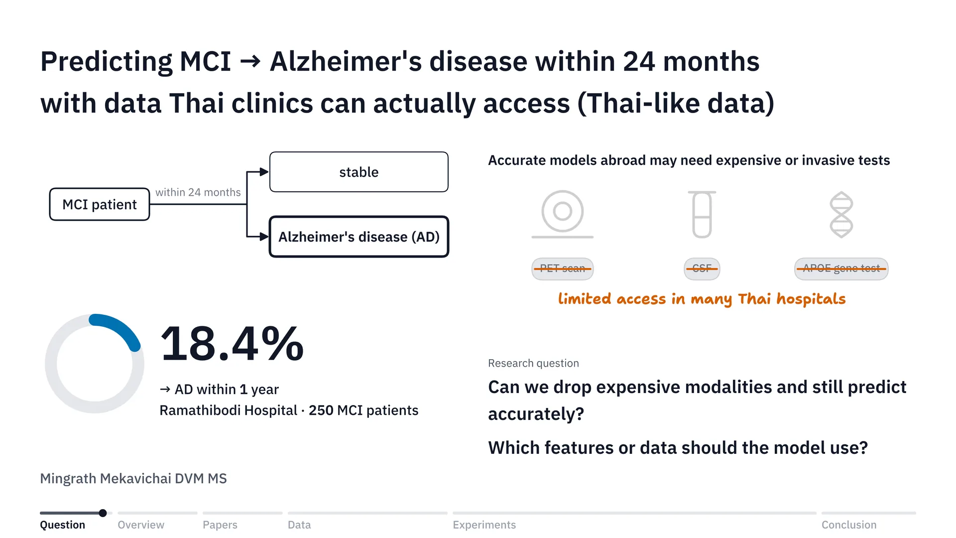
In Thailand, access to the modalities for diagnosing disease may not exist in every hospital, and there may be quite a lot of people who don’t even have the money, or the means, to access those modalities. One of the systems that needs a lot of modalities for diagnosis is the nervous system, and one of the conditions we see a great deal in neurological disease is Alzheimer’s.
There’s one thing about Alzheimer’s that I find quite interesting: the progression from mild cognitive impairment, or MCI, to Alzheimer’s disease, or AD. A study from Ramathibodi Hospital[1] found that out of about 250 patients, as many as 18.4% progressed from MCI to AD (the study counted conversion to dementia, not to Alzheimer’s specifically) within 1 year — that’s about one in five. If we can tell who will progress from MCI to AD, doctors can plan treatment better, right?
But to make a model predict this progression accurately, most studies abroad have to use expensive modalities or invasive diagnosis, whether that’s a PET scan, CSF, or testing for the APOE gene, and many hospitals in Thailand still have limited access to these modalities.
So it would be really great, wouldn’t it, if we could cut out the expensive modalities or the invasive diagnosis and still predict progression from MCI to AD just as accurately. The question is: can we? And if we can, what features would we need? Or put simply, what data do we need for the model’s prediction? And that is where the project I did in Brain Code Camp 2026 came from.
Overview: from data to a set of tools
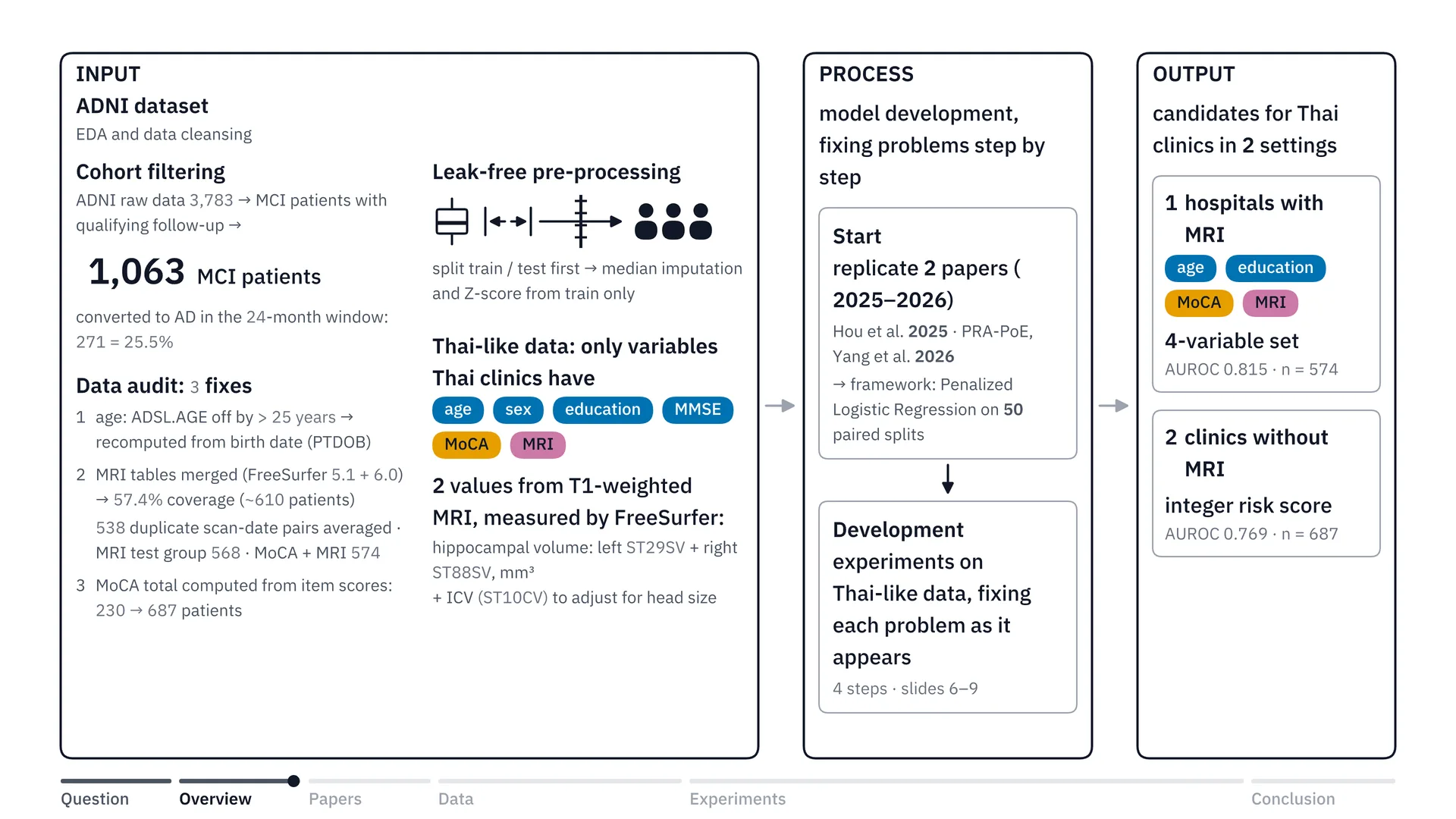
First, let’s look at the overview of the project. It starts with choosing a dataset, right? Okay, which dataset are we going to use for this project? And since Thailand doesn’t have many public datasets, or doesn’t have a public dataset we could use to train a model to look at progression from MCI to Alzheimer’s, right, we used the ADNI dataset[6] instead. ADNI is data on Alzheimer’s patients in North America. Once we had the data, we did EDA and cleansed it — screening patients, fixing ages and so on, which I’ll go into later — and we merged the tabular MRI data and recalculated the MoCA score. All of this was getting the dataset ready to train the model, and it came out as 1,063 MCI patients in total.
Then we did the pre-processing while preventing data leakage, meaning we don’t let bias in, by keeping the train and test sets clearly separate. And we scoped it to only what Thailand has, so I labelled it Thai-like data: age, sex, years of education, MMSE and the MoCA score, plus T1W MRI, which gives two values: hippocampal volume and ICV. The T1W values I used are computed with a program called FreeSurfer, which measures the volumes and puts them into a table as numbers. The values we use are hippocampal volume and ICV, which is intracranial volume.
Let me expand a little on how a scan turns into a number. A T1 MRI image is three-dimensional, like a whole loaf of bread cut into thin slices. Each slice is made of tiny cubes about 1 millimetre across, called voxels. FreeSurfer automatically colours in which voxel belongs to which part of the brain, then counts the voxels that are hippocampus, on both the left and the right side, and gives a volume in cubic millimetres. ADNI has already done this step, so we just take the resulting table and use it.
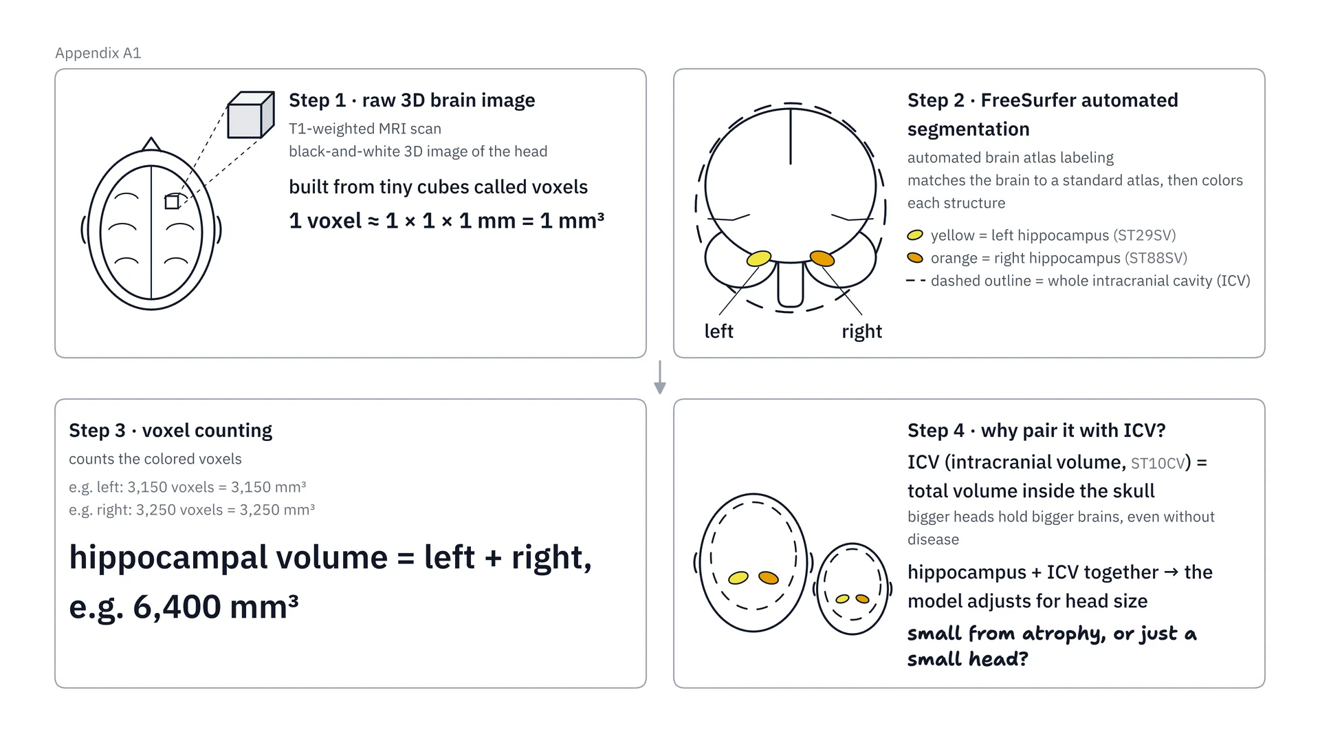
Going through the illustration step by step, it starts with step 1: a T1 MRI image is a three-dimensional image made of tiny cubes about 1 millimetre across, called voxels. Then in step 2, FreeSurfer automatically colours in which voxels are the left hippocampus and the right hippocampus, and outlines the skull cavity, which is called ICV. Once the colouring is done, in step 3 we count the voxels of both hippocampi together, giving a volume in cubic millimetres. And in step 4, the reason we always have to pair it with ICV is that people with bigger heads already have bigger brains. ICV helps the model tell whether a small hippocampus is small because it has really atrophied, or because the head is small. ADNI has already produced these numbers; where a Thai hospital would get these values is the first limitation I talked about in the limitations section below.
Then, for model development, we looked for papers that did something similar to us, meaning cutting out modalities, especially ones focused on the ADNI dataset. We found two papers: Hou et al.[2] from 2025 and PRA-PoE[3] from 2026. In the end we chose penalized logistic regression, using 50 paired splits — I’ll tell you the details in the next section — and then developed the experiments on Thai-like data.
And finally, the Output: we get a set of options, or candidates, for two settings, with MRI and without MRI, which I’ll talk about further below.
What we learned from the 2 source papers
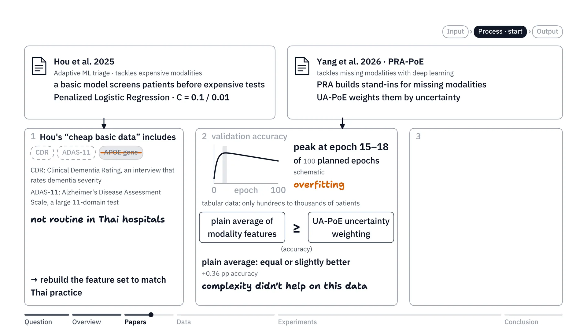
Before we look at data cleansing, let me briefly tell you why we trained the model this way. At first, the goal of our project was to try cutting out the expensive modalities, right? So we looked for papers close to ours, and found Hou’s 2025 paper on adaptive triage: using a basic model to screen patients before sending them on to the expensive tests. There was also another paper, by Yang, on PRA-PoE, which tries using a deep learning model to help predict patients who haven’t had every modality tested.
So I tried replicating both papers on the ADNI dataset I actually had, following their methods. The very first thing I found was that the word cheap, or cheap basic data, in their paper doesn’t mean the same as really cheap in our country. They included CDR, the Clinical Dementia Rating, which we don’t do here, and ADAS-11, which we don’t do either, and the APOE gene was also included in their cheap set. But in Thai hospitals, we don’t routinely test these things. So if we’re going to group the data into features, we should group them to match the reality in Thailand too.
The second thing: when we started replicating Yang’s paper on our dataset, we saw that the deep learning model we built was overfitting at about epoch 15–18. The accuracy on the validation set peaked around those epochs, and training further didn’t make it any better, because our data only ran to hundreds or a few thousand (looking back, that peak also coincides with the end of the learning-rate warm-up at epoch 15, so it is indirect evidence for choosing a simpler model: it proves neither that the model was overfitting nor that the small sample caused it). That is exactly the overfitting problem. So I decided, okay, deep learning may not suit us very well, and I cut the deep learning part and didn’t take it further, because it didn’t help much on this dataset.
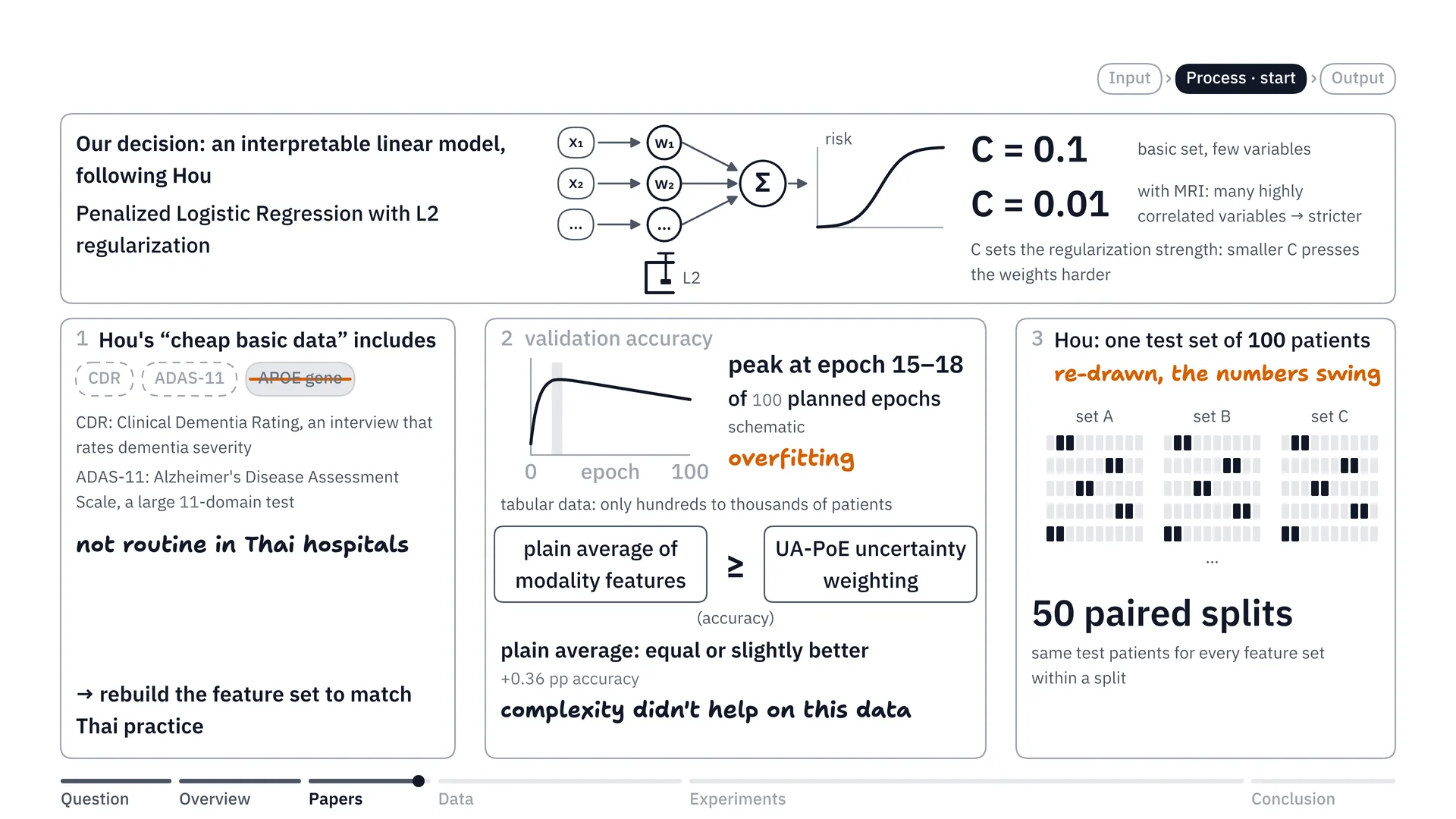
In the end we decided, okay, let’s build an interpretable linear model instead. Put simply, we use a linear model and we can open it up and look at the weights inside, to see which features matter more or less — what the weights look like. That’s basically Hou’s recipe. We made penalized logistic regression our main model. Penalized logistic regression is like doing logistic regression but adding L2 regularization, to help stop the model from piling too much weight onto any one value, because we don’t want it to overfit. As for C, we set it at 0.1 for the basic information, because that set has only a few variables, and we gave C = 0.01 to things like the MRI data, because brain data has many variables that are highly correlated, and we didn’t want the model to overfit on them too much.
And finally, the third thing: Hou’s paper evaluated on a single test set of 100 patients, and when we re-drew it, the numbers swung a lot. So we did the evaluation with 50 paired splits: randomly splitting the data into train and test 50 times, so that the numbers don’t depend on the luck of a single draw.
Preparing the data: screening patients, fixing bugs and preventing data leakage
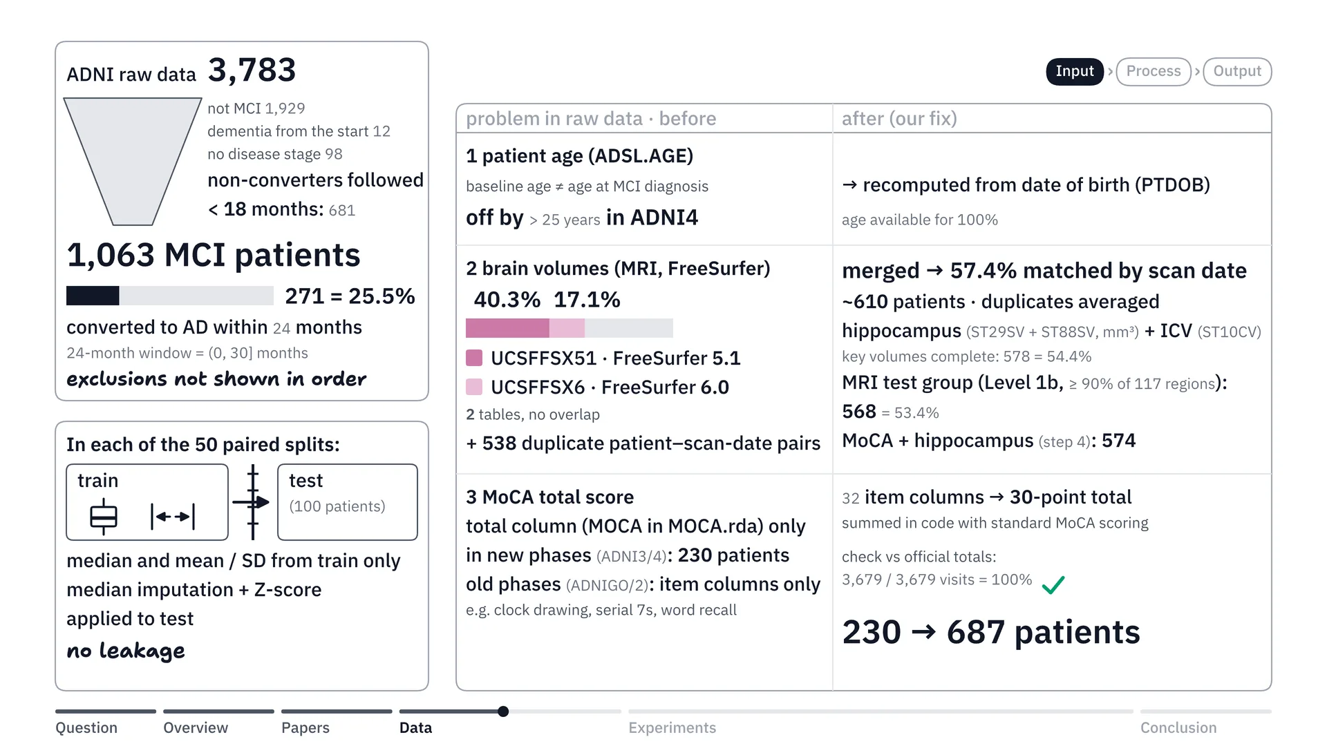
Once the experimental framework was settled, we did EDA and data cleaning on the ADNI data we downloaded, which has 3 parts.
The first part, we did cohort filtering. The data has 3,700-odd people, right? We removed people who weren’t MCI, and people who didn’t convert to AD but were followed for less than 18 months, so that people who dropped out midway don’t get mixed in. In the end we’re left with 1,063 MCI patients to include, and in this group a total of 271 converted to AD, or 25.5%, which matches the statistics.
The second part, we did a data audit, and we found 3 problems. The first was age. Because the ADNI dataset records age at first enrolment (strictly, the age in that table is the baseline age of the current ADNI phase), not when the person started developing MCI, some people had values that were quite far off, so we recalculated it.
The second was the tabular MRI table. This is where they ran the MRI images through FreeSurfer and turned them into tables in the ADNI dataset, and there are 2 versions. The first is FreeSurfer 5.1, and it turned out its data was only 40.3% complete, while FreeSurfer version 6.0 was at 17.1%. So we merged these two tables and matched up the scans, which brought completeness to 57.4%, or put simply about 610 people (57.4% is the share whose scan dates could be matched; 578 people had complete volumes). We also averaged 538 pairs of duplicate scans from the same day, then picked the people with complete brain data, which gave us an MRI test group of 568 people, and a group with both MoCA and hippocampus of 574 people.
Lastly, the MoCA score. In ADNI’s tables, patients tested in the newer phases have a column with the total out of 30 already added up, but that’s only 230 patients. For patients in the older phases, the total column hadn’t been added up for them. So we went exploring in the ADNI database and found that they kept the results item by item, all 30 columns (strictly, 32 scored item columns that add up to a 30-point total) — say, can you draw the clock, or subtracting 7 at a time, things like that. So we recalculated: we wrote a formula and first computed it for the newer-phase patients who already had a total, and found, oh, okay, it’s correct. Once the formula was right, we used it to convert the older-phase patients too, which gave 687 patients in total, all recalculated and revalidated.
And the last part is preventing data leakage. Data leakage is when data from the test set secretly leaks in while we train the model, which makes the results look better than they really are — like students seeing the exam before they sit it. So we prevented it like this: in every one of the 50 splits, once we split train and test, the numbers used to prepare the data — whether the median used to fill in missing values, or the mean and SD used for Z-score scaling — are computed from the people in the train set only, and then the same numbers are applied to the test set. So the test set is like new patients the model has truly never seen.
Choosing features that match Thai clinics
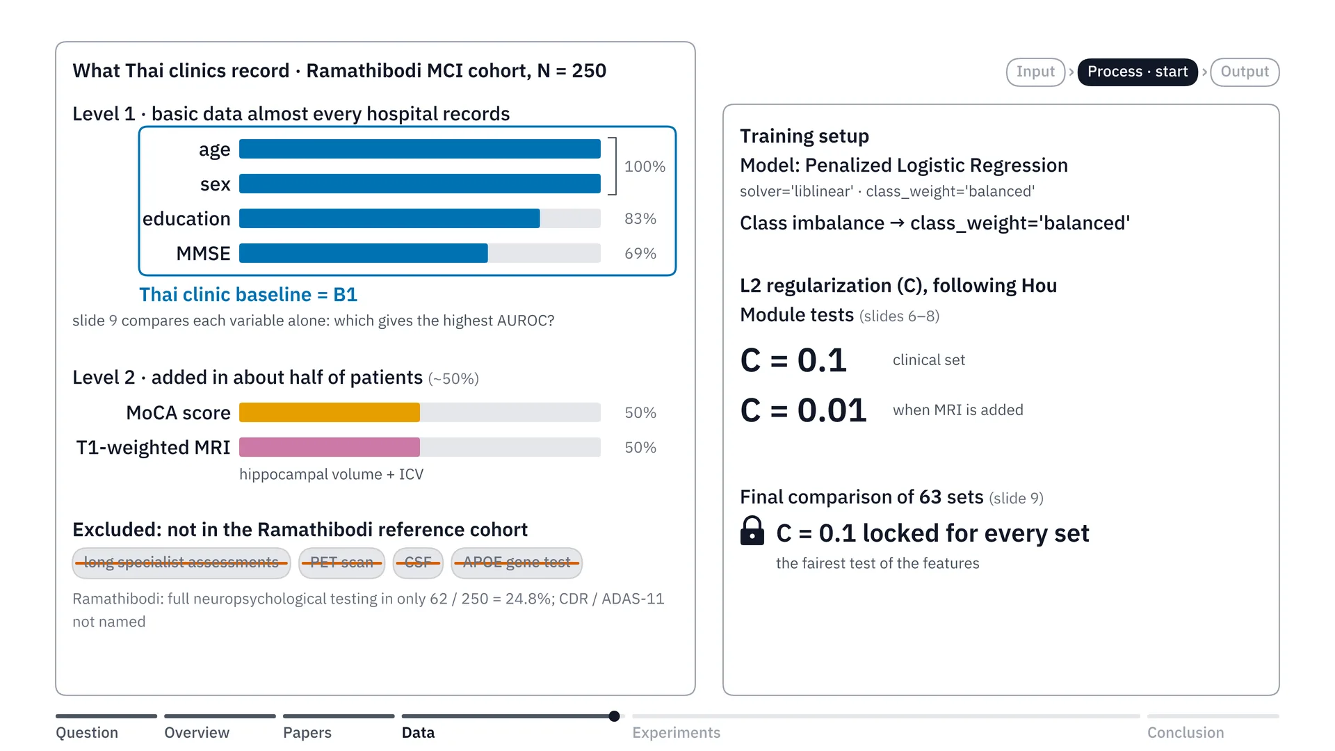
Now that the data was cleaned and settled, right, the next step was choosing features to match the setting of Thai hospitals, to use for training the model.
We drew on the Rama Hospital study of 250 MCI patients I mentioned earlier, which led us to split Thai features into 2 tiers. The first tier is truly basic data that almost every hospital already collects: age, sex, education and the MMSE score. Actually, in step 4 we’ll see which one gives the model the highest AUC.
AUC, or in full AUROC — think of it as a pair-guessing game. Take a pair of patients: one will progress to AD, the other won’t. Then have the model point to who is at higher risk. AUROC is how often the model points correctly, across all the pairs. 0.5 is the same as tossing a coin; 1 means it points correctly on every pair. The closer to 1, the better.
But for now we put these in first, and we named this basic clinical data set B1, to keep things simple. The second tier is what Thai hospitals can additionally test in about half of patients: the MoCA score and MRI, focusing first on T1-weighted MRI. As for the assessments that take a long time, and also PET scans, CSF taps or gene tests like APOE — which aren’t in the Rama Hospital reference cohort — we chose not to use them to train the model.
As for how we trained the model, as I said, we used penalized logistic regression with class weight set to balanced, to deal with the imbalanced classes, and we used L2 regularization following the recipe of Hou’s 2025 paper: C = 0.1 for the clinical data and C = 0.01 for the MRI group of data, in the stage where we tested the modules separately. In the final stage, where we compared 63 patterns — I said we’d compare every one — we locked C at 0.1 for every set, to measure the effect of the features as fairly as possible.
Step 1: is basic data enough, and how much does MRI help?
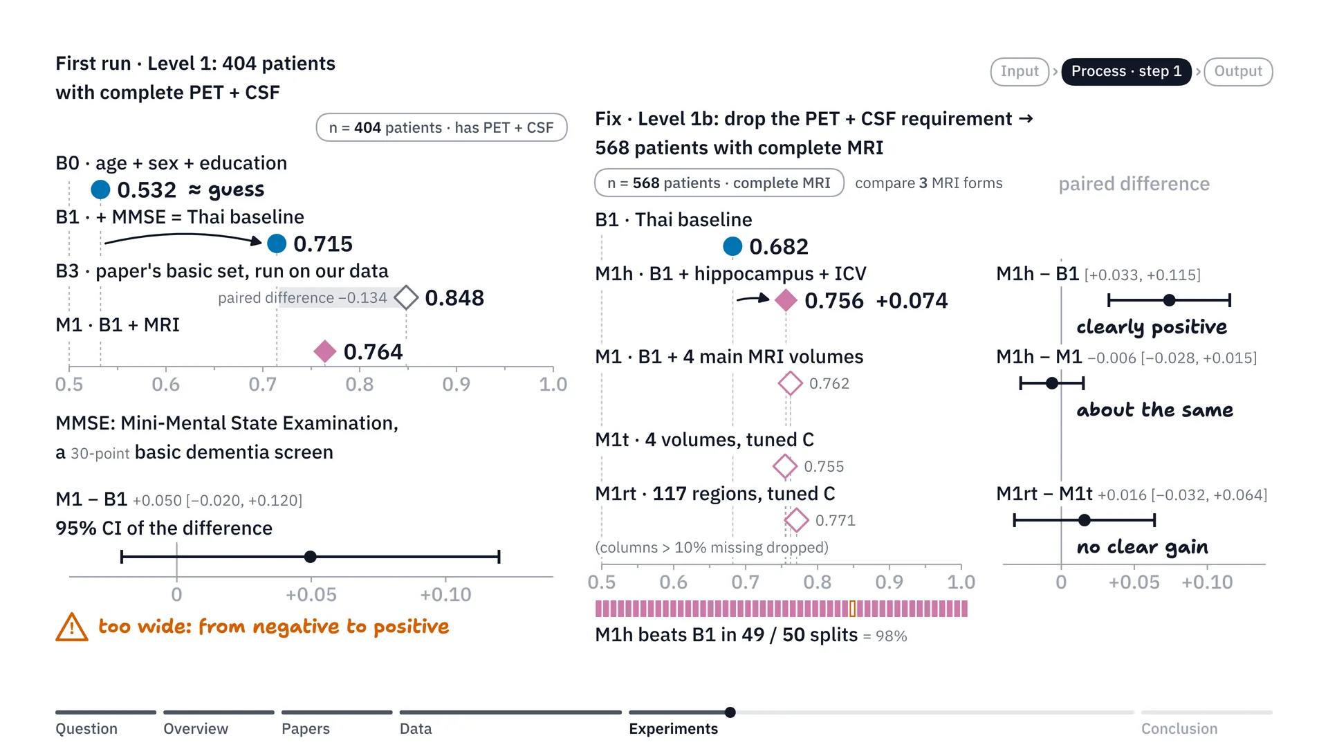
Now let’s look at the results of the first experiment. When we first ran the model, we used B1 data from n 404 people. These 404 were selected because they had complete data like PET scan and CSF. And we found that if we used only age, sex and education, we’d get AUROC of only about 0.53, which is about a coin toss. But when we added MMSE, which is a test, the AUROC jumped up to 0.715. That’s still lower than the paper’s basic set run on our data, which got about 0.848 — quite a big difference, as you can see.
Another problem we hit in the first run: when we put in the MRI values, which we hoped would help move AUROC up, it did move up to 0.764, but the confidence interval had a range that was too wide. The range of the difference swung from negative all the way to positive, which made us feel the conclusion still wasn’t clear — whether adding MRI really makes the model more accurate.
So I looked again and ran it another round, but this time — in the end we’re probably not interested in PET scan and CSF anyway, right? Because in Thailand they’re not widespread diagnostics; they’re not modalities among the features we’d put in anyway. So I wanted to increase n. In the second round we removed the PET scan and CSF condition, which got n up to 568 people.
Then we compared how much MRI data is enough, trying 3 ways. The first way, we used only hippocampus volume, which is the memory part of the brain, paired with ICV, or intracranial volume, which is there to adjust so that people with small heads and big heads can be compared. The second way, we used 4 MRI volumes, adding the entorhinal cortex — the part of the brain next to the hippocampus and one of the first places Alzheimer’s starts to destroy — and the ventricles, the fluid spaces in the brain, which get bigger as brain tissue atrophies. And the third way, we pulled in all 117 regions across the whole brain, and tuned C as well. C is the strength of the penalty on the model’s weights that I told you about earlier (strictly, it is the inverse: the smaller the C, the stronger the penalty); tuning means that instead of locking the value, we let the model try many values in the train set and pick the best one itself. Then we looked at which way worked best.
The result was very clear: in the group of 568, adding just hippocampus and ICV pulls AUROC from 0.682 up to 0.756, or put simply an increase of a full 0.074, winning 49 of 50 rounds. And it gave results very close to using the 4 main regions, while putting in all 117 brain regions did not clearly add accuracy over the 4-main-region model with tuned C. So we concluded: then just hippocampus paired with ICV is enough.
Step 2: trying to send only the people who need it for MRI
Now, from the first step’s results, we can see that adding MRI features helps AUC a great deal. So we wanted to try mixing in the idea from the paper that did triage: we test everyone with the basic B1 set first, and then send for an MRI scan only the cases the model isn’t very confident about.
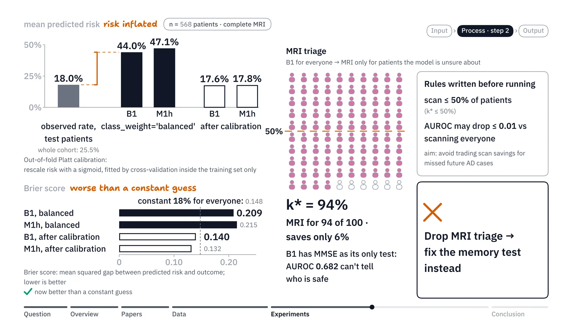
But when we ran it, it turned out that in the subgroup with complete tests, the real disease rate was about 18%, but when we gave the classes balance, the side effect was that the model’s average predicted risk went up to 44–47%. Now, the Brier score, which measures the error between the risk the model predicts and the real outcome — when the model over-predicts at 40-something percent, the Brier score comes out quite bad, even worse than guessing that everyone has the same 18% risk.
So we tried fixing it with out-of-fold Platt calibration on the train set. Platt calibration takes the skewed risk and puts it through an equation that rescales it to match the real proportion of disease. And out-of-fold means we split the data inside the train set and take turns doing the calibration, without mixing in the test set at all, to pull the risk scale back. The result is that the average risk the model predicts comes back to about 17.6–17.8%, which is much closer to the real disease rate of 18% than at first, and the Brier score dropped from 0.209 to just 0.140.
But in the end, there was still a point that stopped us going further with this plan. Even though we tried to calibrate the risk until it was okay, when we tried picking people to send for MRI, we set the rules before the run: we must send no more than 50% for scans, and we won’t allow AUROC to drop by more than 0.01, or in other words, it may point wrongly on no more than 1 extra pair in 100 pairs. Because we don’t want anyone to get a missed diagnosis, right?
When we ran it, we found we still had to send 94% of patients for scans, or put simply it saved only 6%. The reason is that the basic B1 model using MMSE doesn’t have much starting accuracy: its AUROC is only 0.682. Put simply, MMSE on its own can’t separate the patients cleanly. When the basic model can’t call who is really safe, it doesn’t dare drop anyone, so it has to send as many as 94% for MRI scans. So I thought, okay, this kind of MRI triage might not work very well, and instead I went to fix the problem at MMSE, this memory test.
Step 3: swapping MMSE for MoCA, and a points table on paper
From step 2, we can see that MMSE is like a bottleneck in the model’s prediction, right? So in this step we focused on: what if we try using the MoCA score instead, in our n of 687 people?
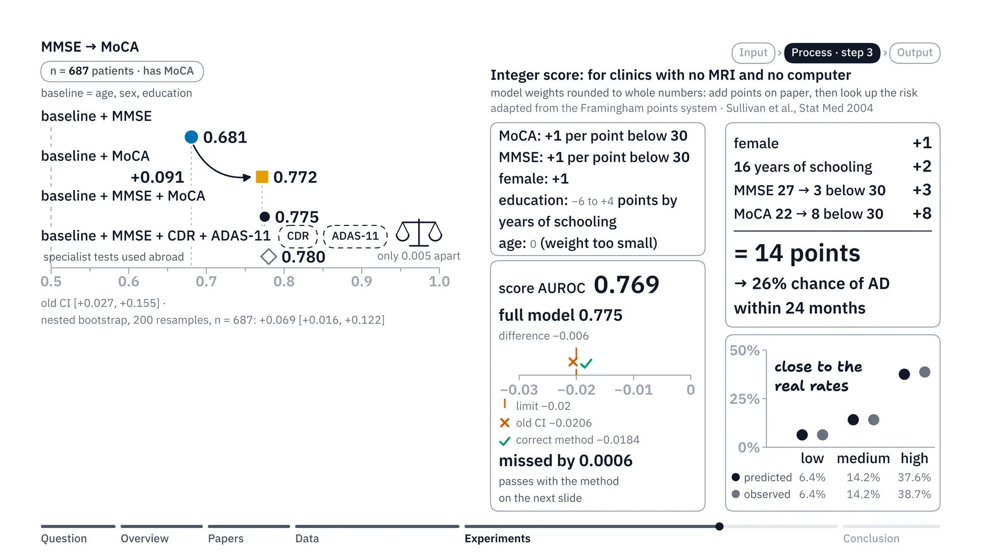
The MoCA score measures executive function in more detail than MMSE. When we used the MoCA score as a feature in the model instead, the result was quite clear: just switching from MMSE to the MoCA score raises AUC, or AUROC, from 0.681 to 0.772. Put simply, it goes up by a full 0.091. And using MMSE together with MoCA gives about 0.775, which is close to the assessment sets used abroad, like CDR plus ADAS-11, whose AUROC is about 0.78. That means for Thai clinics without MRI, just switching to the MoCA score closes almost all of this prediction gap (more precisely, MMSE + MoCA reached 0.775 against 0.780 for CDR + ADAS-11, a difference of +0.005 [−0.036, +0.046]: no clear difference was detected, which is not proof that the two are equal).
Then I thought further: but up-country clinics don’t have MRI, and they might not be able to sit and run our model, right? So how could a doctor in an up-country clinic use this model? So we tried taking the hard decimal weights in the model’s equation, rounding them to integers, and making a points table. I call this the integer score. It’s the same way of thinking as the Framingham points system that Sullivan and colleagues published in 2004[4], so that doctors can calculate it on paper. For example, say the MoCA score or MMSE is however many points below 30: you add 1 for each point, or if it’s a woman you add 1, something like that.
Let’s just do an example. Say it’s a woman: 1 point. She studied for 16 years in total, which means she finished a bachelor’s degree: 2 points. She scored 27 on MMSE, 3 short: 3 points. MoCA score 22, 8 short: 8 points. Add them up and you get 14, and the doctor can take the number 14 and look it up in our table right away: this patient has a 26% chance of Alzheimer’s within 2 years (up to 30 months including visit tolerance).
When we checked the accuracy of this number table, meaning the accuracy of the integer score, it turned out the AUROC was as high as 0.769 — only a tiny drop from the model’s 0.775. And when we split the patients by points into 3 groups — low, medium and high risk — the risk percentages our table predicted matched the percentages of patients who actually got sick in all 3 groups (close rather than exact: 37.6% vs 38.7% in the high group). There was just one small catch: when we checked the statistical criterion with the old CI formula, it missed by a hair, just 0.0006, before we switched to the correct statistical method in the next step, and then this points table passed the criterion.
Step 4: trying all 63 combinations, fixing the statistics, and choosing the best-value set
Now we come to step four: we took all 6 groups of variables and arranged them into 63 patterns. I fixed C at 0.1, the same for every set, and ran the comparison on the same group of 574 patients.
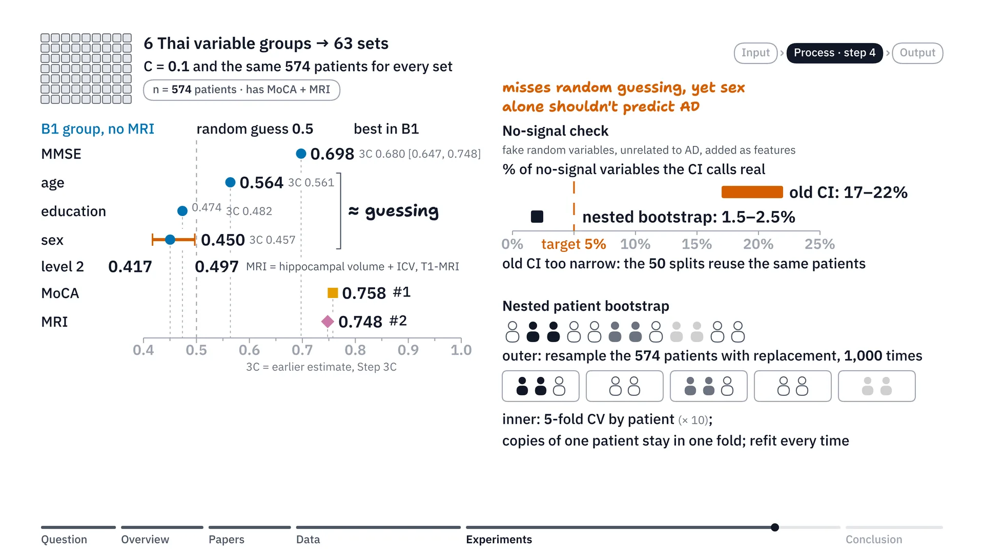
As I said when choosing the features: say we could put in only one single feature, which one would give the model the highest AUC? Looking at the results in the figure, it’s quite clear. In the basic group, B1, the group without MRI, if we put in only age, AUC is just 0.564, which is very low, basically no different from guessing. Or sex alone is only 0.450. These basic data on their own are just random guessing. The one that still makes the B1 group best is the MMSE score alone, which keeps this group’s highest AUC at 0.698. But if we also count the second-tier variables like the MoCA score and MRI, number one is the MoCA score alone, with AUC at 0.758, and number two is hippocampal volume extracted from T1 MRI images, at 0.748.
There’s one interesting point here: with the single variables, we notice an anomaly. In the model with only the sex variable, we see that the old 95% confidence interval runs from about 0.417 to 0.497, right? It doesn’t cover 0.5, which it normally should, because 0.5 is a coin toss. So the 95% interval for sex should cover 0.5 too, because sex shouldn’t be able to predict the disease, right?
So I suspected the old formula must have some problem, and I added one more test: a no-signal check. Put simply, I randomly created a fake variable of random numbers, numbers with no relationship at all to Alzheimer’s, and tried using them as a feature in the model. By the rules of statistics, this should pass by fluke — put simply, give a false positive — only about 5% of the time. But it turned out that with the old confidence interval formula, it says these random variables actually work as much as about 17–22% of the time. The reason is that the patients are the same group of patients, swapped back and forth and overlapping, so the old formula computes an error range that’s narrower than reality.
So we tried a new kind of resampling: a nested patient bootstrap. To picture how it works, we do it in two nested layers. In the outer layer, we randomly draw the list of 574 patients with replacement, or sampling with replacement, afresh from the start, 1,000 rounds in total (in the final runs, 200 rounds for the main scans of the variable sets and the score recheck, and 1,000 for the boundary checks, each round with 10 × 5-fold cross-validation inside; the later mentions of 1,000 here, the 1,000 new groups and the thousand rounds, refer to the boundary checks). In each round, some patients are drawn more than once and some aren’t drawn at all — as if we simulated going out and collecting 1,000 new groups of patients.
Inside, once we have each round’s list of patients, we split it with 5-fold cross-validation — that is, into 5 piles — separating train and test again inside that round. The rule is that if a patient is drawn several times, every record of that patient must always go into the same pile, so the same patient can’t leak back and forth between train and test. Then we train a new model and evaluate it separately in every one of the thousand rounds. This method cut the false positives from about 20% down to just 1.5–2.5%, which is within an acceptable range by the rules of statistics.
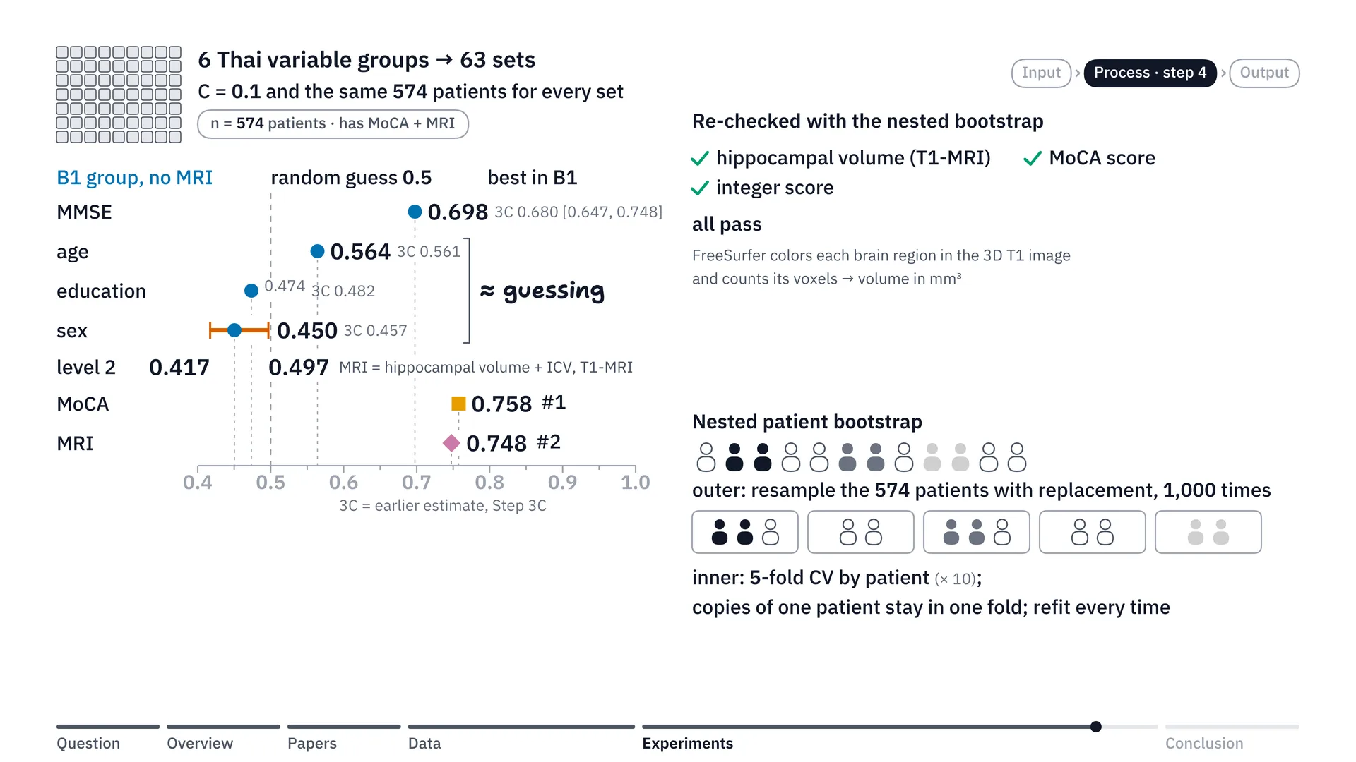
Now when we took the statistical method we thought should be right and re-ran everything, we found that hippocampal volume from T1-weighted images and the MoCA score values still pass the criterion as before, and the integer score that missed the criterion by 0.0006 in step 3 does pass when checked with the new method.
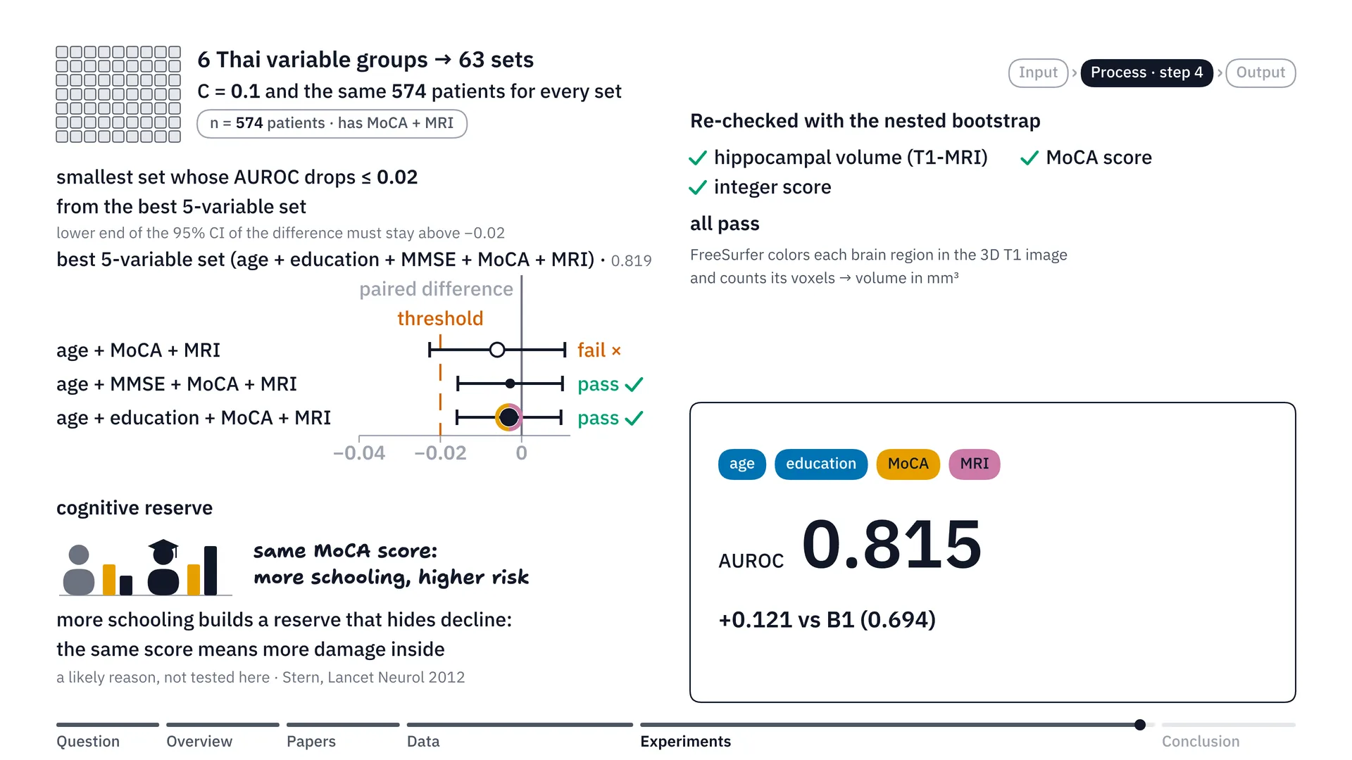
Finally, choosing the best-value combination of variables for Thai hospitals. Instead of cramming in every variable and making doctors run lots of tests, we set a rule: if we want to cut the variables down to as few as possible, we’ll allow AUC to drop from the set with everything in (strictly, the best 5-variable set, 0.819; all 6 variables gave 0.817) by no more than 0.02, or put simply, it may point wrongly on no more than 2 extra pairs in 100 pairs. Checking through, if we use only 3 variables — age, MoCA and MRI — the accuracy still drops a little more than 0.02 (more precisely, the mean drop was only 0.0060; it is the lower bound of the 95% confidence interval, −0.0226, that crosses −0.02). But when we move up to 4 variables, we find 2 sets that pass: adding MMSE, or adding years of education.
Years of education has a very interesting point. If you look at years of education on its own, it can barely predict the disease at all. But when it’s used together with the MoCA score in the model, it turns out that if two patients score the same on MoCA, the one with more education has a higher risk of Alzheimer’s than the other (this was seen in the integer score, with both MMSE and MoCA held equal). The likely medical reason is cognitive reserve[5] (one possible explanation, which this work did not test), the brain’s reserve capital: people who studied a lot have brains that can prop up or mask illness better than people who studied little. So when a highly educated person’s test score falls to the same level as someone with little education, it means the brain tissue inside has likely deteriorated a lot, to the point that their original capital can’t hold up any more, and so they have a higher chance of declining into Alzheimer’s within two years (up to 30 months including visit tolerance).
So we chose this 4-variable set — age, years of education, MoCA score and brain volume from MRI, which is hippocampal volume with intracranial volume — as the main model for hospitals with an MRI machine. Because this set gives AUC of 0.815, shooting up from the original basic B1 set, which got only 0.694, an increase of a whole 0.121. And in practice, the doctor can just ask the patient for their years of education while taking the history, without wasting time making the patient take an MMSE test that may overlap with the MoCA score.
Summary: what we got for Thai clinics
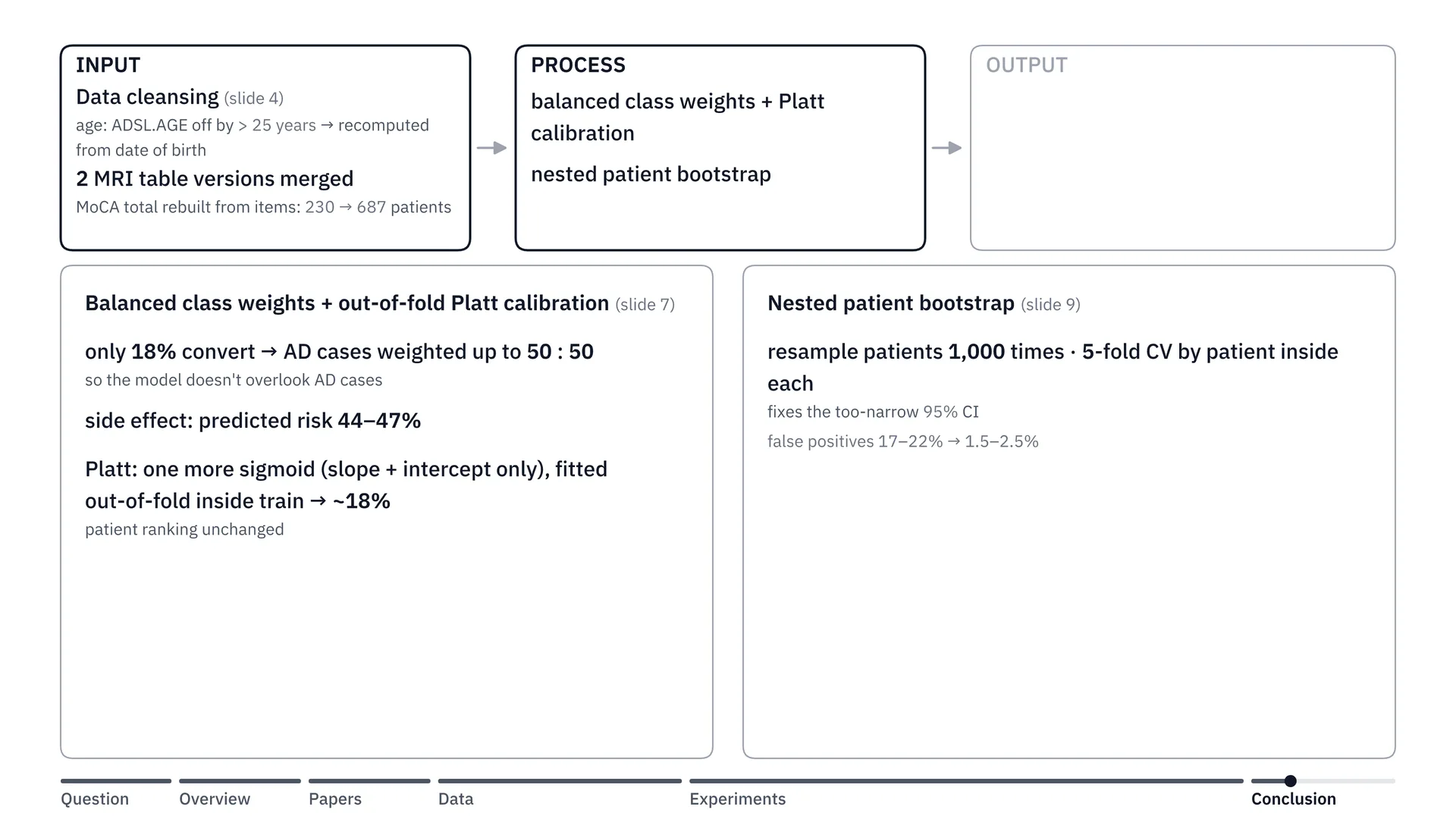
Let’s look at the overview of our project once more. Okay, we used the ADNI dataset, and we did various cleansing: fixing the ages that were off, merging the separate tabular MRI data together, and the MoCA score that was missing, we recalculated it.
Step two is the process of developing the model. At this stage we hit a problem with balanced class weight. Because in our data the share of patients who changed from MCI to Alzheimer’s was 18% (in the test sets of the 568-patient MRI group; in the whole cohort it is 25.5%), when we trained the model we used balanced class weight, telling the model to multiply up the importance of the Alzheimer’s group until it balances at 50 to 50, so the model doesn’t overlook the people who are sick. But the side effect is that when the model sees the sick as half, the risk percentages it predicts shoot above reality, to 44–47%. So we corrected it with Platt calibration. Put simply, Platt calibration is like a scale that reads too heavy every time. We don’t need a new scale, we just set the needle straight. Whoever is heavier than whom still lines up the same, but the numbers come back to the truth. So the average risk came back to 18%, and we set the needle from the train data only, without peeking at the test side.
Step three, covered above, was testing MoCA in place of MMSE and building the paper integer score. And step four is that we switched to the nested patient bootstrap. Put simply, it’s like going back in time to collect a new set of patients 1,000 times (in the final runs, 200 times for the main scans and 1,000 for the boundary checks). And each time, we put the model through an exam with 5-fold cross-validation: splitting the patients into 5 piles, letting the model learn from 4 piles and then sit the exam on the remaining pile, rotating through every pile, with the same patient always in the same pile, so no one sees their own exam in advance. Doing it this way, the confidence interval isn’t narrower than reality like with the old formula. And all of this gave us a set of options for Thai clinics in two settings.
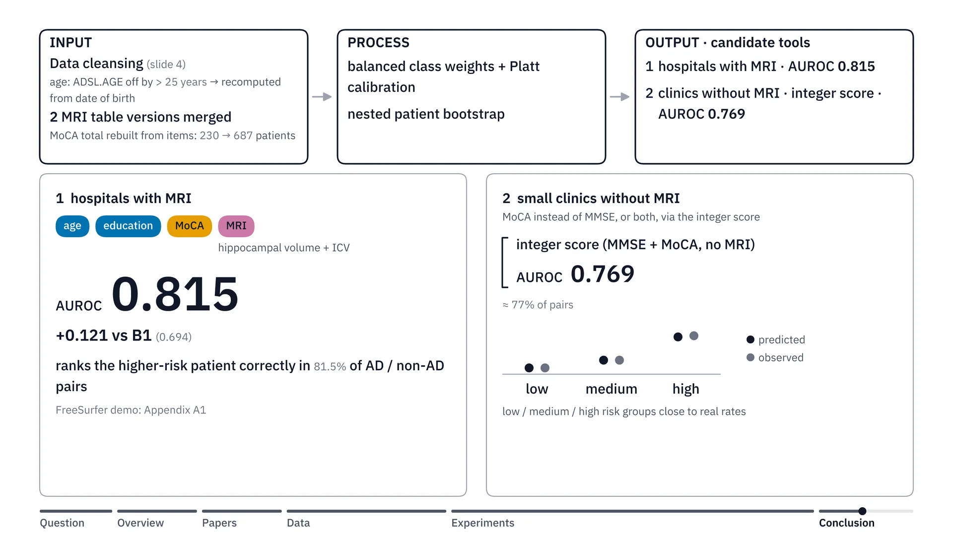
The first setting is hospitals with MRI. The right set is the data group with 4 variables, which is what I chose: age, years of education, MoCA score, and hippocampal volume paired with ICV, as I said earlier. This data set gets AUROC of 0.815, up from the basic B1 set by a full 0.121.
And the second approach is for small clinics without an MRI machine: we can switch to the MoCA score instead of MMSE and use it together with the integer score, which we can calculate right on paper (the integer score itself uses both MoCA and MMSE, plus sex and years of schooling). This puts AUC at about 0.769, an option that’s easy to use and gives risks close to the real data.
For doctors: what the integer score is and how to use it
This section is written for doctors who really want to try this points table, especially up-country clinics with no MRI, or no computer to run a model. You can read it in two minutes.
What is the integer score?
The integer score is a points table on paper. It needs no computer and no MRI. We took the decimal weights in the model’s equation and rounded them to whole numbers, adapting the Framingham points system that Sullivan and colleagues published[4]. You just add up the patient’s points, then look the total up in the table, and you get the risk of the outcome the table was built to predict. The outcome: an ADNI clinical diagnosis of dementia within 30 months of the first MCI visit (a 24-month target plus 6 months of tolerance), not Alzheimer’s confirmed by biomarkers. Below, “this outcome” means exactly this.
What data do you need?
- MoCA score
- MMSE score
- Sex
- Years of schooling
All of these come from a routine visit. You need both MoCA and MMSE. Age is not needed, because age got 0 points in every one of the 50 splits.
Enter the MoCA total before the extra education point (the +1 that the MoCA form adds for few years of schooling): the model was built on totals out of 30 without that point, and the table already scores schooling on its own.
How to use it, step by step
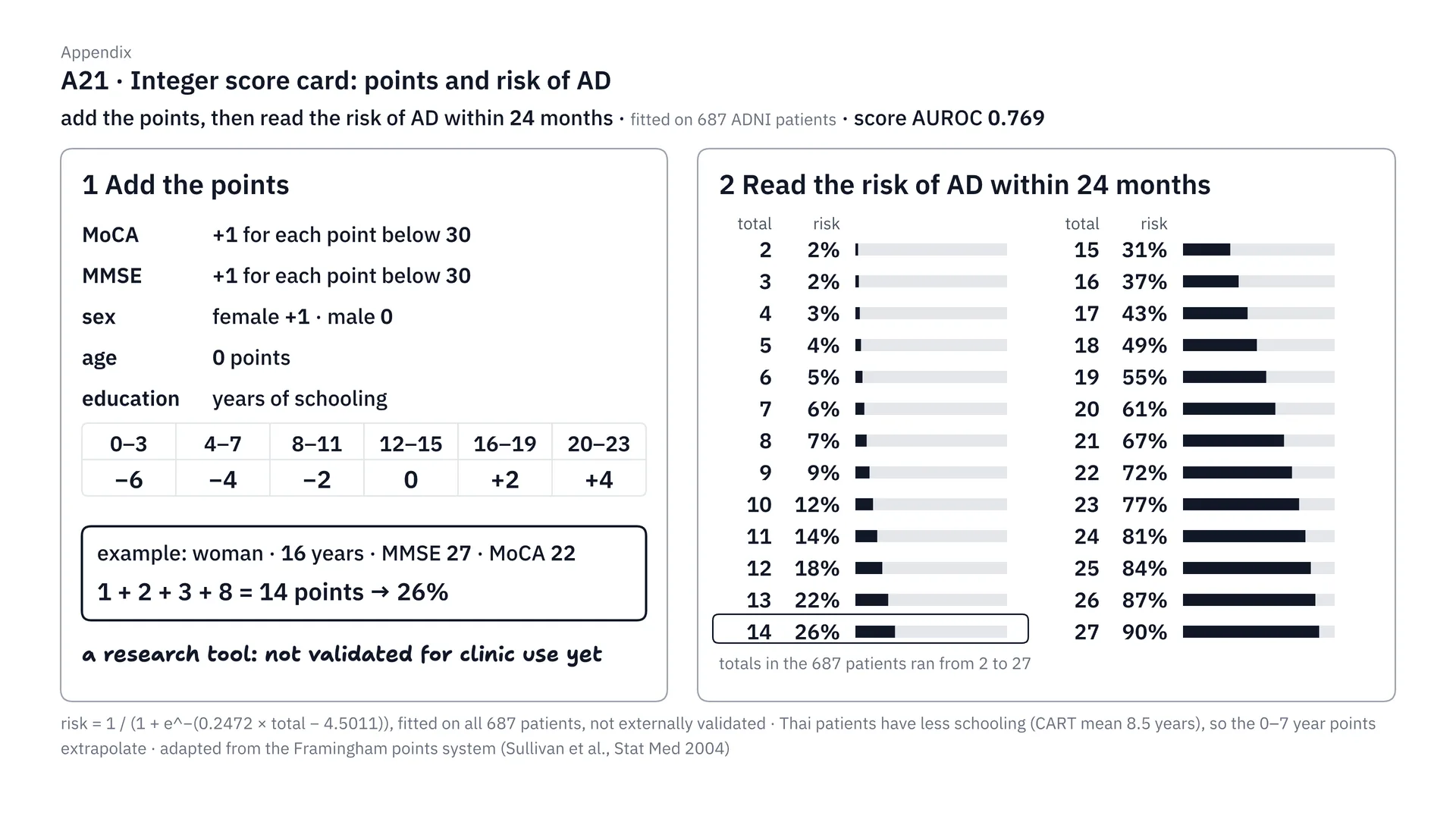
This is the full integer score table. Step one, add the points: for MoCA and MMSE, however many points short of 30, add that many. Women add 1. Education adds or subtracts according to the band of years studied, and age gets no points. Step two, take the total and look it up in the table on the right. Like the example below, which gets 14 points: that’s a 26% risk within 24 months (up to 30 months including visit tolerance). This method is adapted from the Framingham points system, but I have to stress that it’s still a research tool, fitted on 687 ADNI patients, and not yet validated in Thai patients.
Step one: add the points
| Input | Points |
|---|---|
| MoCA | +1 for each point short of 30 |
| MMSE | +1 for each point short of 30 |
| Sex | female +1, male 0 |
| 0–3 years of schooling | −6 |
| 4–7 years of schooling | −4 |
| 8–11 years of schooling | −2 |
| 12–15 years of schooling | 0 |
| 16–19 years of schooling | +2 |
| 20 years of schooling (the most ADNI records) | +4 |
| Age | 0 |
ADNI records schooling only up to 20 years, so values above 20 are outside the data, and the table has no rule for them.
More schooling earns more points. That sounds upside down, but it’s the pattern from step 4: if two patients have the same MMSE and MoCA, the one with more schooling has the higher risk (cognitive reserve is one possible explanation).
Step two: look the total up in the risk table (the risk of this outcome)
| Total | Risk | Total | Risk |
|---|---|---|---|
| 2 | 2% | 15 | 31% |
| 3 | 2% | 16 | 37% |
| 4 | 3% | 17 | 43% |
| 5 | 4% | 18 | 49% |
| 6 | 5% | 19 | 55% |
| 7 | 6% | 20 | 61% |
| 8 | 7% | 21 | 67% |
| 9 | 9% | 22 | 72% |
| 10 | 12% | 23 | 77% |
| 11 | 14% | 24 | 81% |
| 12 | 18% | 25 | 84% |
| 13 | 22% | 26 | 87% |
| 14 | 26% | 27 | 90% |
The totals of the 687 patients used to build the table ran from 2 to 27. If a patient’s total falls outside this range, the table has no data behind it.
Example (made up, not a real patient): a female patient (+1), 16 years of schooling (+2), MMSE 27, 3 short (+3), MoCA 22, 8 short (+8). Total 1 + 2 + 3 + 8 = 14. The table gives a 26% risk of this outcome.
How good is it?
- AUROC about 0.769, only a little below the full model’s 0.775. Its 95% confidence interval, 0.722–0.816, is the original estimate over 50 splits. The later patient-bootstrap recheck supported the score’s AUROC non-inferiority to the full model (lower bound −0.0184 against the −0.02 margin); calibration was not rechecked. Think of the pair-guessing game from the feature section: 0.5 equals a coin toss, and 1 means pointing correctly on every pair.
- When patients are split into 3 groups by their total, the risk the table predicts is close to the observed rate of this outcome in all three groups. The largest gap was 1.1 percentage points, in the high-risk group (37.6% vs 38.7%).
| Group | Table predicts | Actual |
|---|---|---|
| Low risk | 6.4% | 6.4% |
| Medium risk | 14.2% | 14.2% |
| High risk | 37.6% | 38.7% |
These three groups were split by the totals of the train patients in each round, so this work does not set a fixed cut-off for how many points counts as high risk. Read the percentage from the risk table above instead.
Limits to know before using it
- This outcome is a clinical diagnosis recorded in ADNI, not Alzheimer’s pathology confirmed by biomarkers, and non-converters followed for less than 18 months were left out. So neither conversion rate behind the table is a general MCI conversion rate: in the full cohort, 271 of 1,063 converted (25.5%), and in the 687-patient pool the score was built on, 128 of 687 did (18.6%).
- The table was fitted on 687 ADNI patients in North America, and the risk for each total was computed on the same patients used to build it. It has not been validated in Thai patients at all.
- Thai patients have far less schooling than ADNI patients: the Thai CART registry mean is 8.5 years (the project report gives this figure without a primary CART citation; it has not been independently verified). So the points for 0–7 years of schooling are extrapolated beyond most of the ADNI data. At the other end, ADNI records schooling only up to 20 years, so the table has no data on anyone above 20.
- Thai clinics use MMSE-Thai 2002 and MoCA-Thai. Their scales are similar, but they are not the same tests that ADNI used.
An invitation to help validate it
The next step of this work is external validation in real Thai MCI patients. If you have MCI patient data (MoCA and MMSE scores, sex, years of schooling, and follow-up on whether and when the patient was diagnosed with dementia) and would like to help validate this table, please get in touch through the Contact section on mingrath.com. I’d be very glad to hear from you.
Limitations
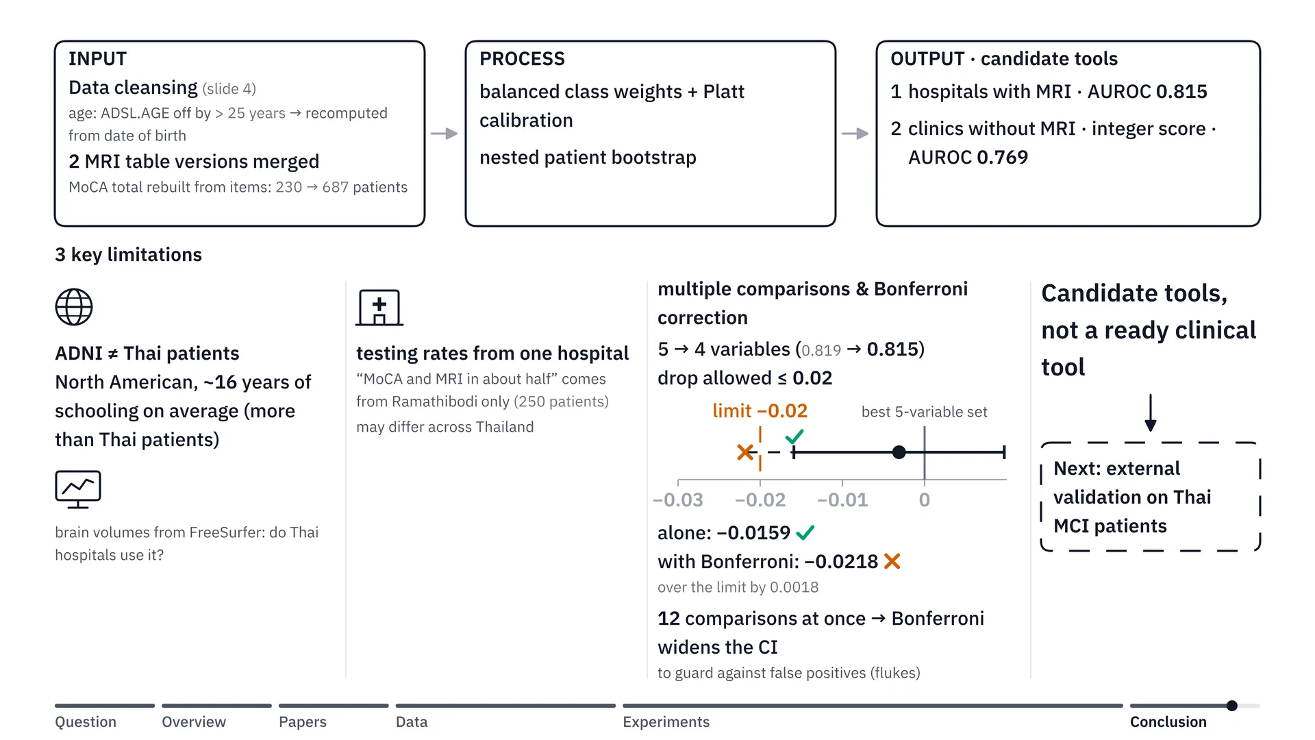
But our work still has 3 limitations. The first is the ADNI dataset we used to train the model. Most of it is data from North Americans, whose average education is about 16 years (an estimate this work did not compute from the cohort; the sources show only that ADNI participants have more schooling than Thai patients, whose CART registry mean is 8.5 years, unverified), which is higher than the average education of patients in Thailand. And then there are the brain volumes we measured with FreeSurfer — we’d need to check whether Thai hospitals use this program.
The second is the testing rates we referenced. For example, we said MoCA and MRI are done in about half of patients; that’s based on a study from Ramathibodi Hospital alone, which means it might not be like this for hospitals across the whole country.
The third and last one: when choosing the 4-variable set in step 4, we set a rule that accuracy must not drop from the full set (here, the best 5-variable set, 0.819) by more than 0.02. Looking at this set on its own, the worst case (the 95% CI lower bound, not a guaranteed worst case) drops only 0.0159 — an easy pass. But at that time we were comparing as many as 12 sets (12 comparisons, or contrast rules) at once, which is like buying many lottery tickets: the more you buy, the more chance you have of winning by fluke. So statistics has a way to compensate, called Bonferroni correction: the more sets you compare, the wider the uncertainty range you have to allow. Once we allowed for that, the worst case (the Bonferroni-adjusted lower bound, also not a guaranteed worst case) dropped 0.0218, just a little past the 0.02 line. That means we still can’t say with full confidence that this 4-variable set is as good as the full set.
Next steps
Because of these 3 limitations, we’re not yet claiming this is a ready-made tool that can be used on Thai patients right away. It’s a prototype toolkit, or candidate tools, that tells us which variables give the best value. The next step is external validation with data from MCI patients in real Thai hospitals.
Thank you, and try it yourself
Thank you to my teacher Dr. Itthi Chatnuntawech (Ajarn Khanun), the TAs P’Gus, Oranatt Chaichanasittikarn, and P’Bank, Nithit Singtokum, the advisers of Group G, and all my friends in Brain Code Camp 2026 of the BrainCode101 programme. If you’d like to look at the results of every model yourself, go to bcc.ohmmingrath.com.
The site gathers the results of every model we tried, with each model’s AUROC.
Frequently asked questions
The questions below come from the backup slides I prepared to answer questions after the presentation, for anyone who wants to go deeper.
Data and preventing leakage
How do we count who "converted to Alzheimer's", and why were 681 people removed?
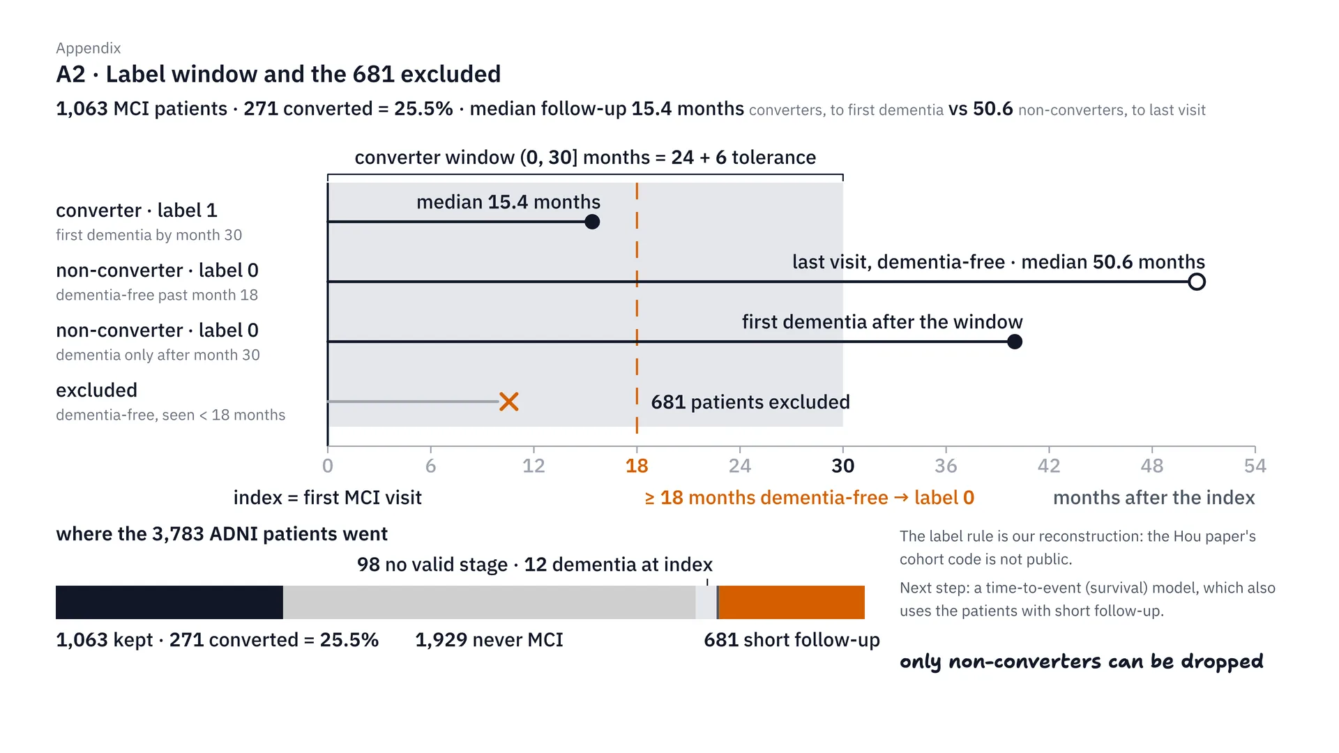
This is our label definition. We count a patient as converting if dementia is first found within 30 months of the date they became MCI — that’s 24 months plus a 6-month margin. Those who don’t convert must have been followed for at least 18 months, because if they were followed for less than that, we don’t know whether they’ll get it later. So we removed 681 people, and we could only remove people who didn’t convert; no one who converted was removed at all. In the end we’re left with 1,063 people, 271 of whom converted, or 25.5%.
In short, the label is an ADNI clinical diagnosis of dementia, not Alzheimer’s pathology confirmed by biomarkers. And because only non-converters with short follow-up were removed, the 25.5% probably runs higher than a general MCI conversion rate, so it should not be read as one.
How did we prevent data leakage, and when were the features measured?
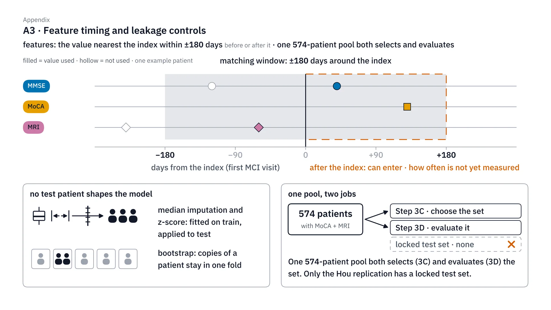
On the timing of features and preventing leakage: for each feature we use the value measured closest to the index date, within ±180 days, which may be a value measured after the index date. I have to admit plainly that this is a bit of a weak point. What actually prevents leakage is that the median and z-score are computed from the train set only, and in the nested bootstrap the same patient must always be in the same fold. One more thing: we used the same 574 patients both to choose the variable set and to measure the results, which may make the results look a little better than they really are.
The teacher asked during the presentation: “Is the z-score computed on everything from the start, or separately for train and test?” The answer is separately. In every one of the 50 splits, we split train and test first, then compute the median used to fill gaps, and the mean and SD of the z-score, from the train set only, and use the same numbers to transform the test set. The test set does not compute its own mean, because in real life new patients come one at a time, and there is no test-set mean to use. This step is inside a scikit-learn pipeline, so it is fitted again in every inner fold too, both when choosing C and when doing calibration. The steps before the split, such as fixing age or adding up the left and right hippocampus, are worked out one person at a time and do not use anyone else’s data.
How different is ADNI data from Thai patients?
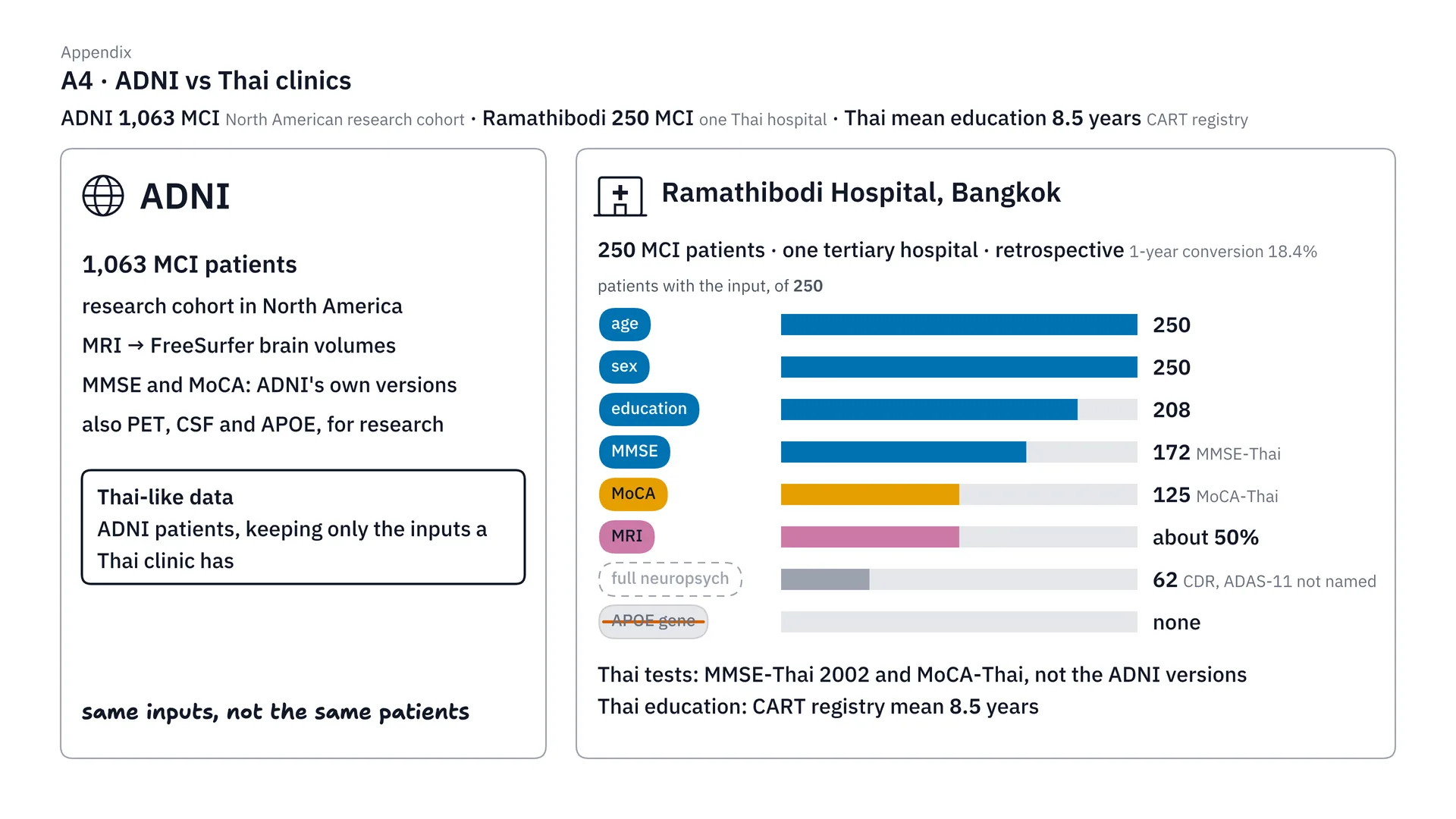
ADNI and Thai patients are not the same. ADNI is 1,063 MCI patients from research in North America. On the Thai side, we reference Ramathibodi’s 250 MCI patients, with education data for 208, MMSE for 172, MoCA for 125, and MRI for about half. What we mean by Thai-like is using ADNI patients but choosing only the inputs Thai clinics have — it doesn’t mean they’re Thai patients. And Thai people studied for only 8.5 years on average (the project report gives 8.5 years as the CART registry mean, not the mean for Thai people in general, and the figure is unverified), much less than in ADNI, so this needs external validation with real Thai data next.
How far can the 0.815 be trusted?
Picking 1 of 63 sets: does the number look better than it really is?
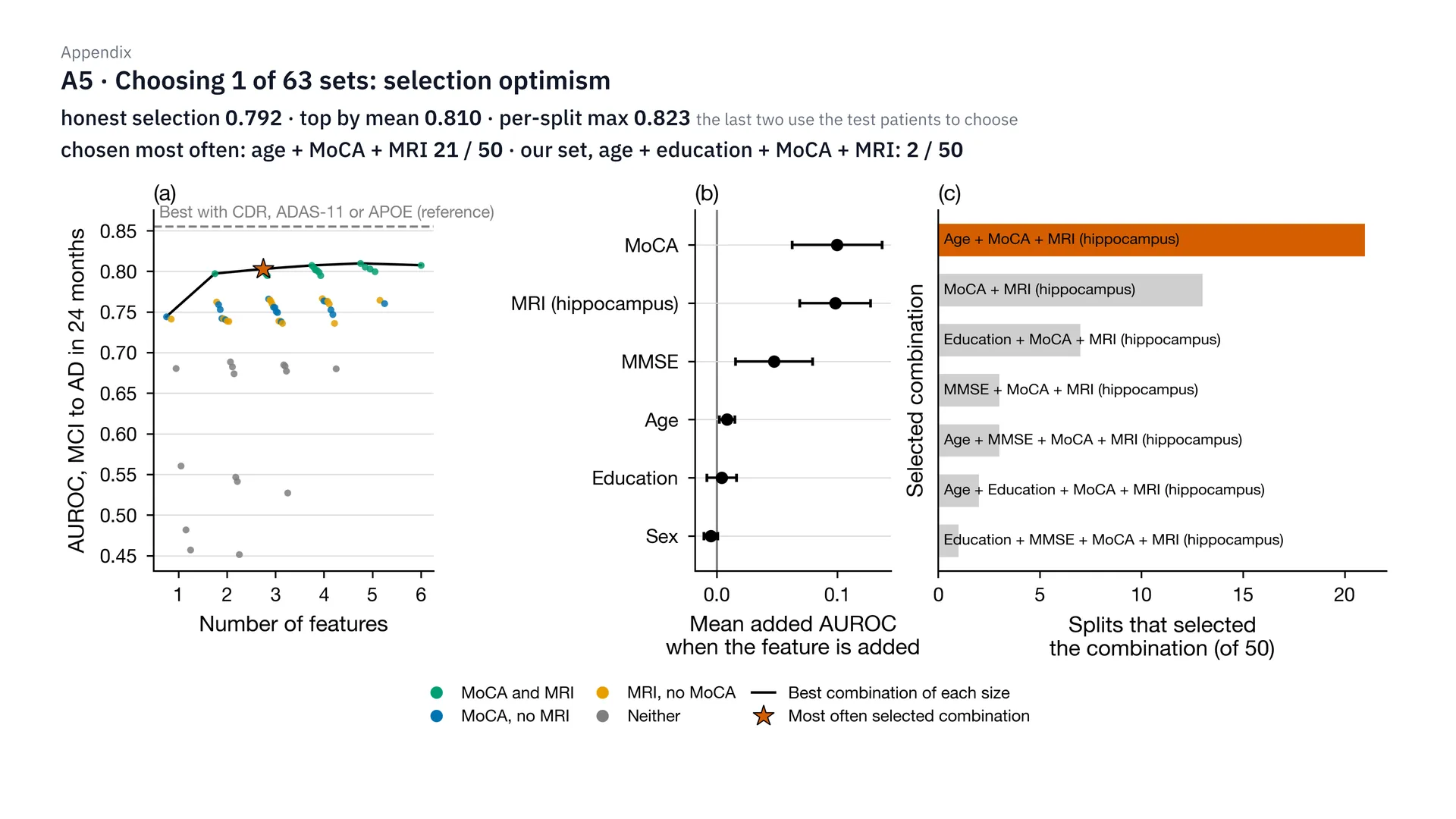
If you ask whether, after picking 1 of 63 sets, the number looks better than it really is, the answer is yes. If we use the test set to choose the best set in each round, we get 0.823. If we choose by the mean, we get 0.810. But if we choose honestly — choosing from the train data only and then measuring on test — it drops to 0.792. The set chosen most often was age + MoCA + MRI, 21 of 50 rounds, while our set with years of education was chosen only 2 of 50 rounds. So 0.815 should be seen as a slightly optimistic value.
How do the "no worse than the best 5-variable set" rule and Bonferroni decide?
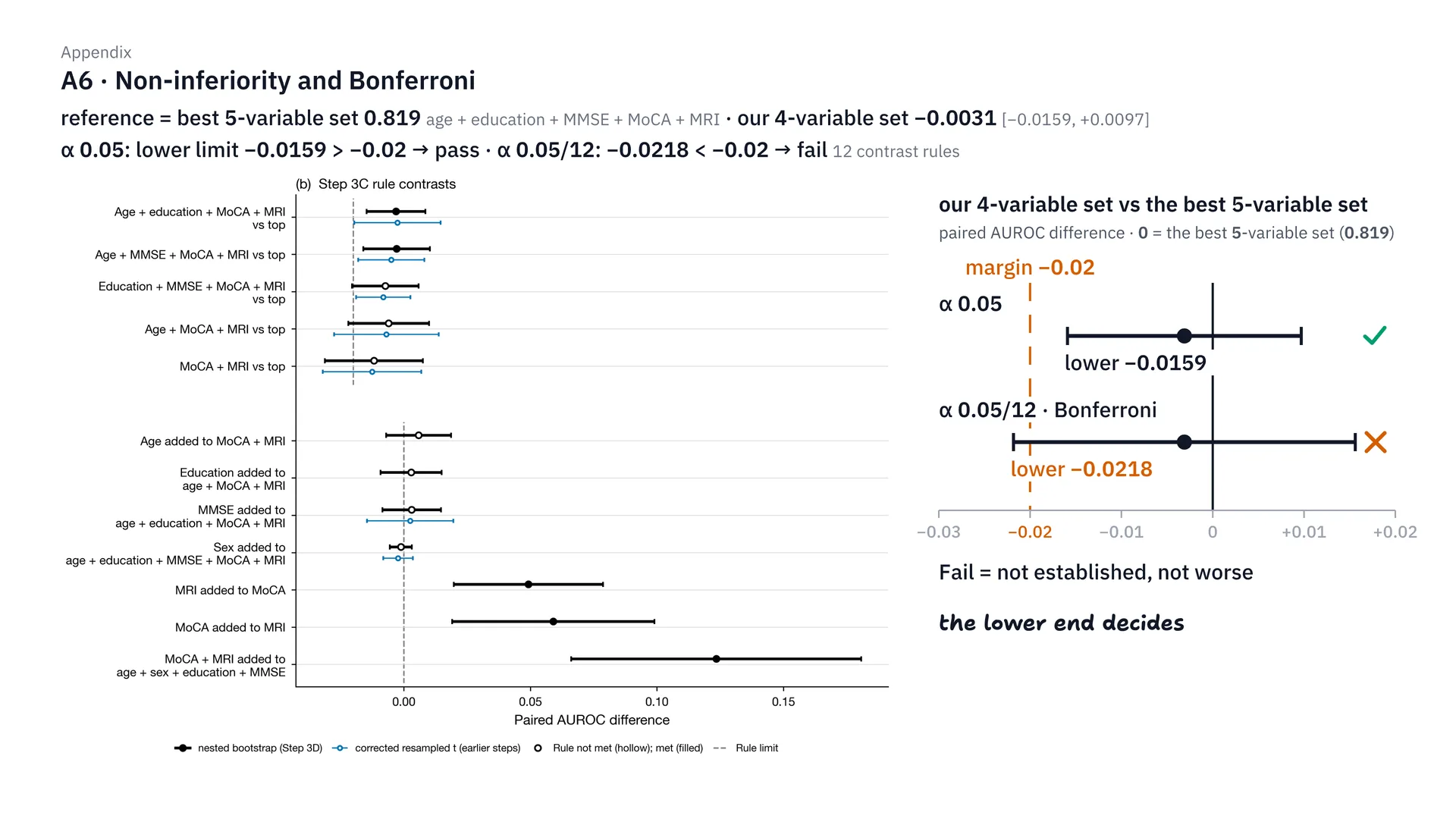
This one is the non-inferiority criterion. We compared our 4-variable set with the best 5-variable set, which got 0.819. The mean difference is only −0.0031, but what decides it is the lower bound of the confidence interval. At α 0.05, the lower bound is at −0.0159, still above the −0.02 line, so it passes. But after correcting with Bonferroni, because we compared 12 sets (12 comparisons, or contrast rules) at once, the lower bound drops to −0.0218, so it fails. That’s why I don’t claim with full confidence that this set is as good as the full set (here, the best 5-variable set), which is limitation 3.
Why did we have to switch to the nested bootstrap?
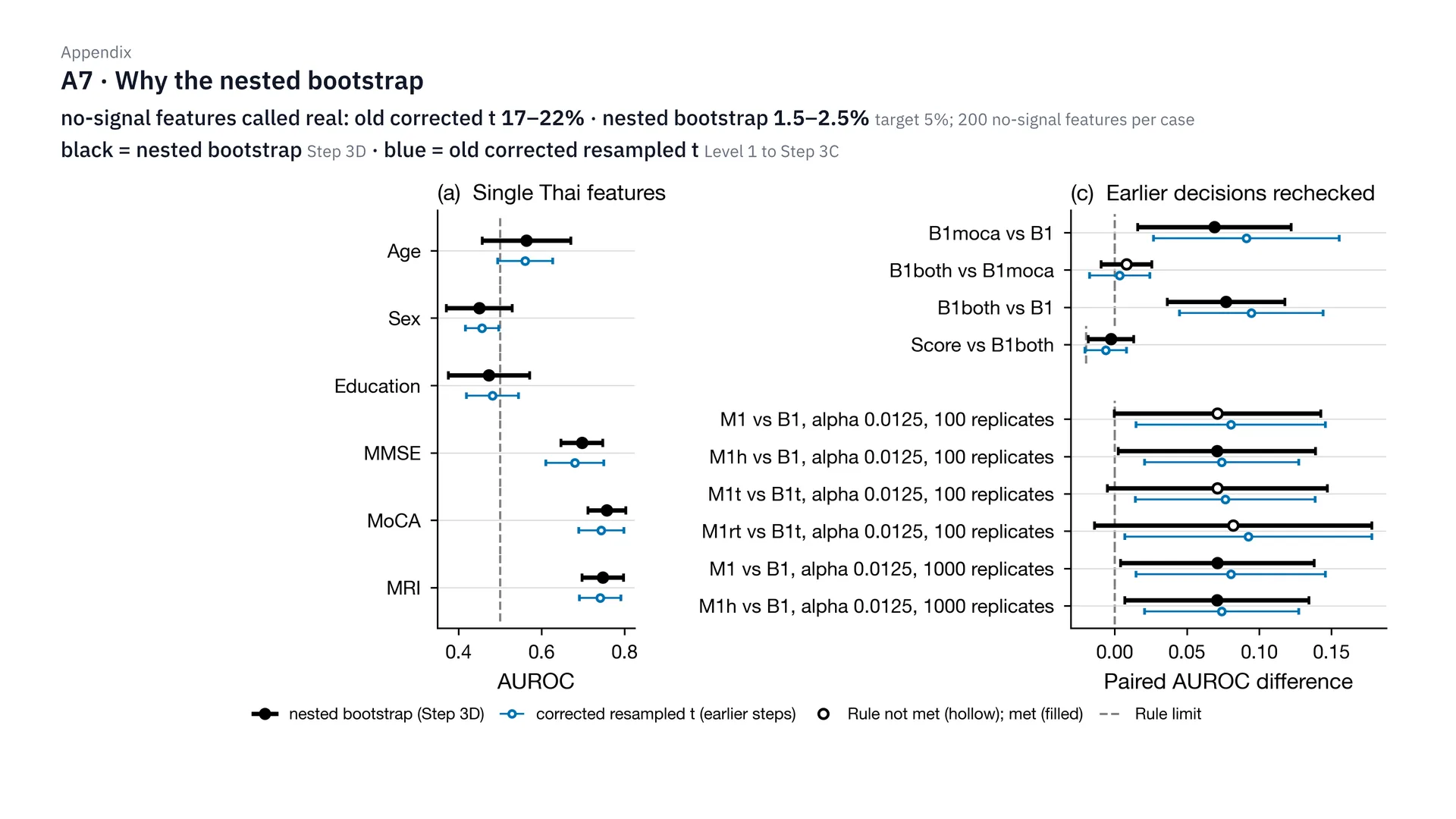
We had to switch to the nested bootstrap because of the result of the no-signal check. We put in fake features with no signal at all, 200 per case. The old formula said they actually worked as much as 17–22% of the time, when it should be only about 5%. But the nested bootstrap leaves just 1.5–2.5%. In the graph, black is the nested bootstrap and light blue is the old formula. This also explains why sex alone got an interval that didn’t cover 0.5 in step 4: because the old formula is narrower than reality.
Did we really try every variable set, and why does the graph say 0.807?
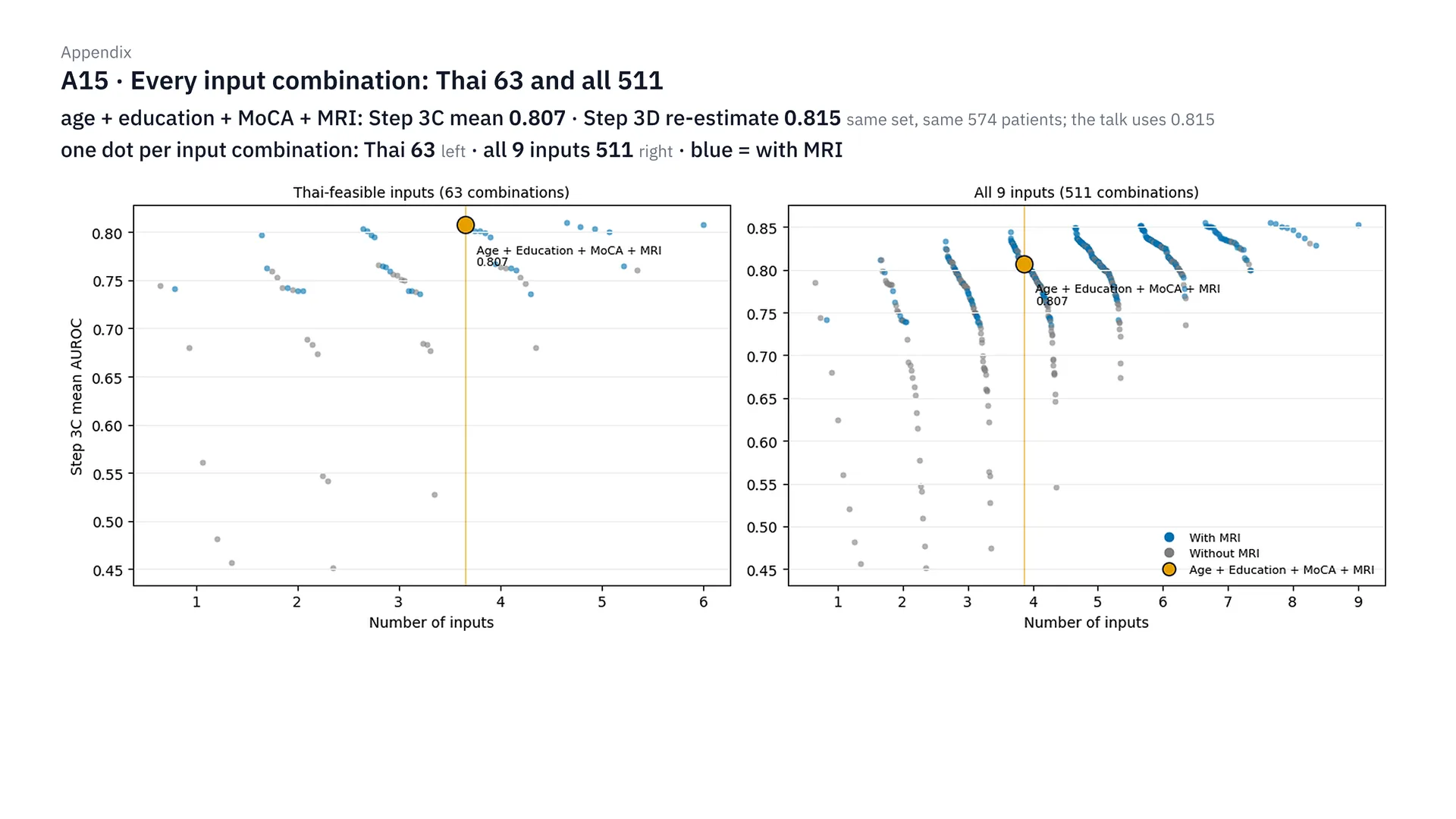
This figure is every variable set we tried. Each dot is one set. The left side is the 63 sets of Thai variables, the right side is the 511 sets from all 9 variables. The light-blue dots are the sets with MRI. And if you ask why the graph says 0.807 but in the main text I said 0.815, it’s because it’s the same set, on the same 574 patients, but 0.807 is the mean from Step 3C, while 0.815 is the value re-evaluated in Step 3D.
In the first round of 404, which patients were the models trained on?
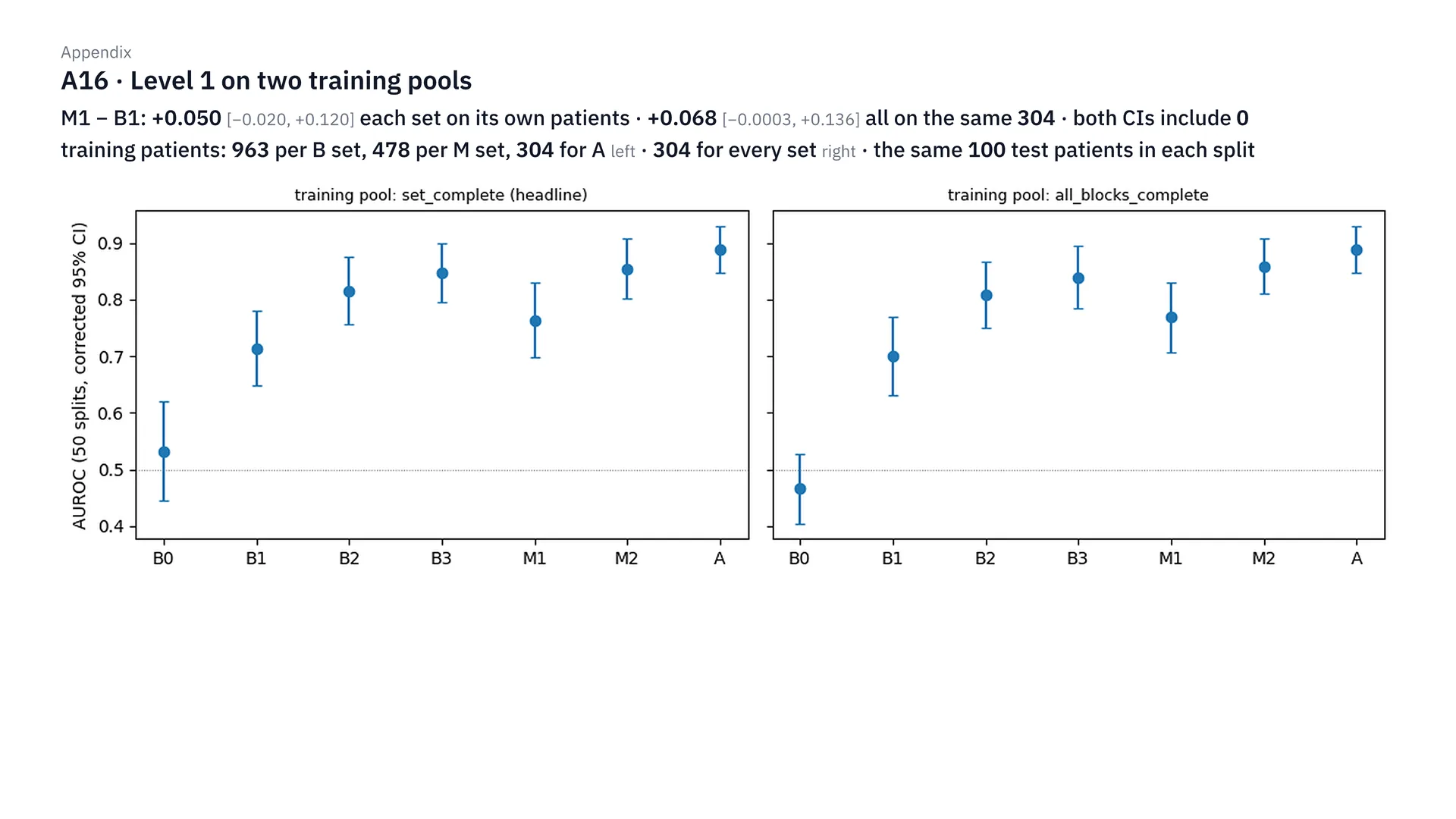
In the first round of 404 people, we tried training two ways. On the left, each set is trained on every patient who has that set’s inputs: set B got 963 people, set M got 478. On the right, every set is trained on the same 304 patients. But both ways test on the same 100 patients in every round. The result is that MRI adds +0.050 and +0.068 over B1, but the confidence interval still covers 0 in both, which is why we expanded to 568 people in round 1b.
MRI, calibration and the points table
Why only hippocampus and ICV?
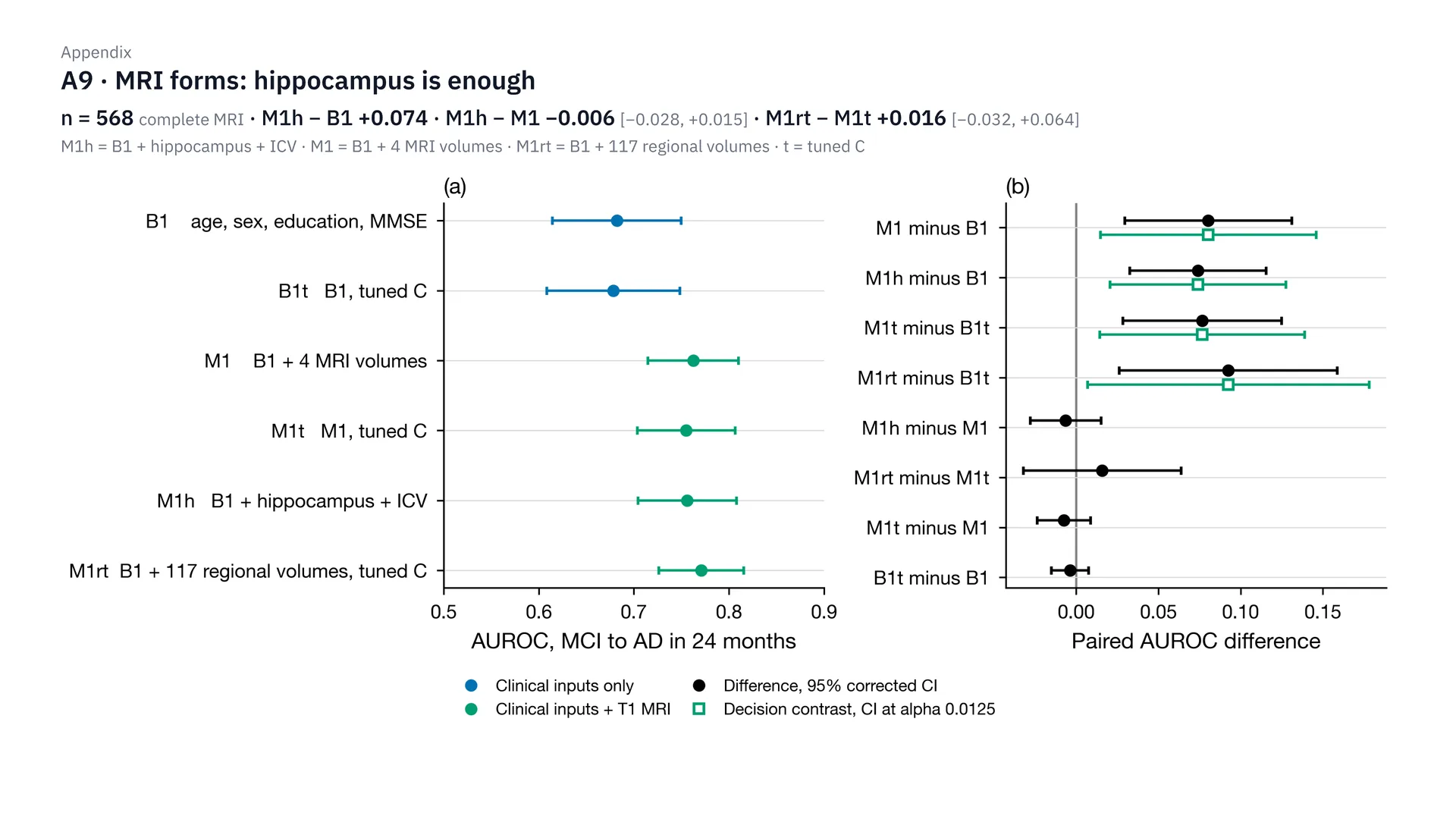
We use only hippocampus paired with ICV because of this result. In 568 people, hippocampus + ICV raises AUROC over B1 by 0.074. Compared with using 4 values, the difference is only −0.006, and the interval covers 0. Using 117 regions with tuned C, which is the t in the graph, adds only 0.016, and the interval still covers 0, so it isn’t clearly better. In short, hippocampus and ICV are enough, which is also simpler for hospitals.
What do the MRI triage graph and sensitivity / specificity look like?
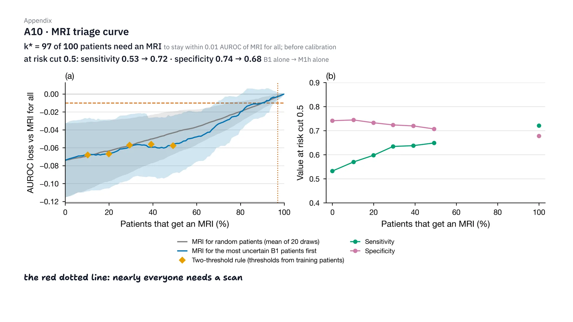
This is the triage graph before fixing calibration. To keep AUROC within 0.01 of scanning everyone with MRI, you’d have to send as many as 97 of 100 people for scans, which is almost everyone. And if you ask about sensitivity and specificity, at risk cut 0.5, adding MRI raises sensitivity from 0.53 to 0.72, but specificity falls from 0.74 to 0.68. We focus on reporting AUROC because these numbers depend on the cut-off we choose.
How much better did calibration and the Brier score get?
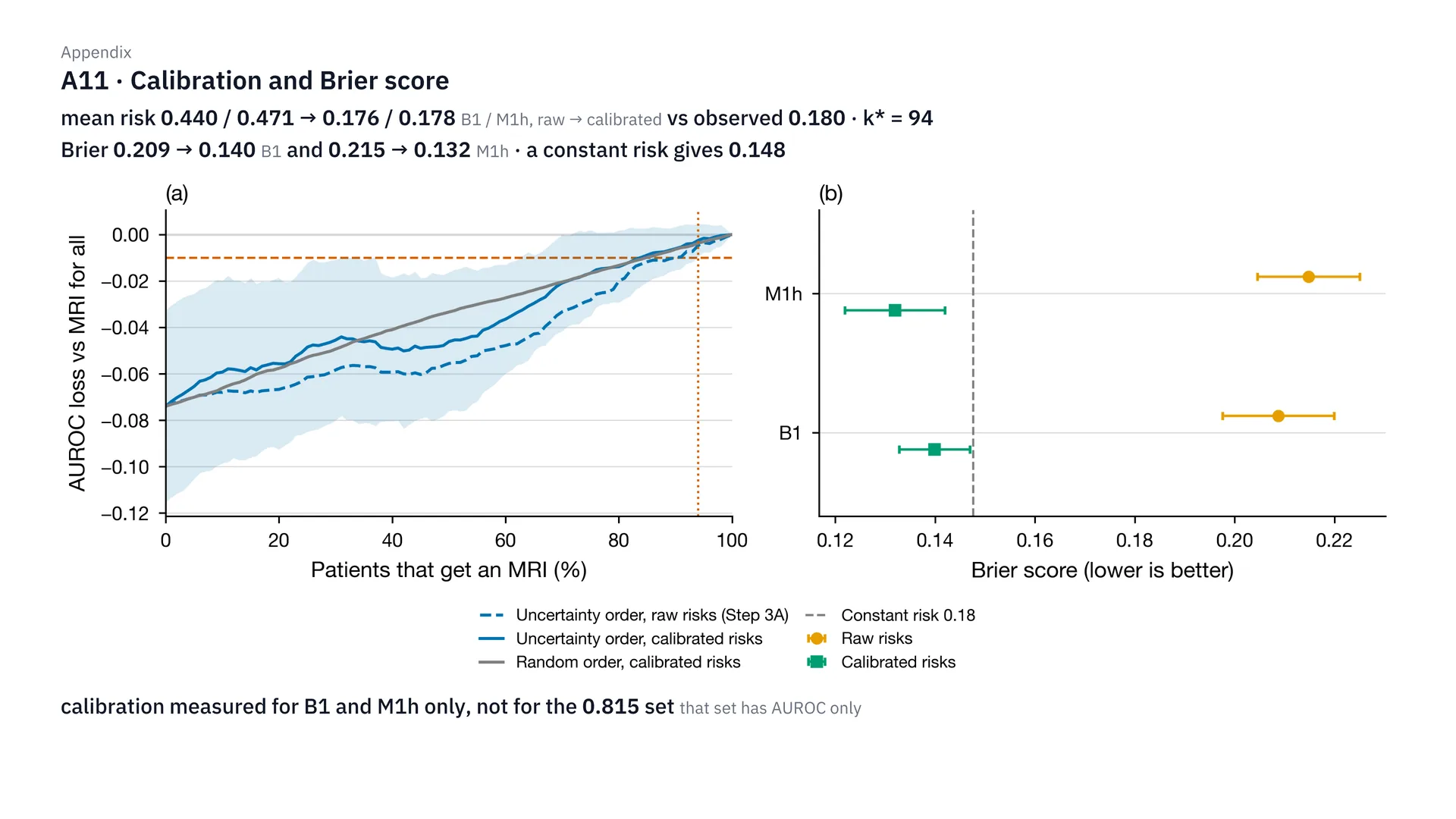
On calibration: with balanced class weights, the average risk the model predicted shot up to 0.44 and 0.47, when the real rate is 0.18. After Platt calibration, it came back to 0.176 and 0.178. The Brier score dropped from 0.209 to 0.140, and from 0.215 to 0.132, which is better than guessing a constant, which gets 0.148. But triage still had to scan 94 of 100 people anyway. One more thing I have to say plainly: for the 0.815 set, we haven’t calibrated the risk yet — there’s only AUROC.
How well do MoCA and the integer score separate risk?
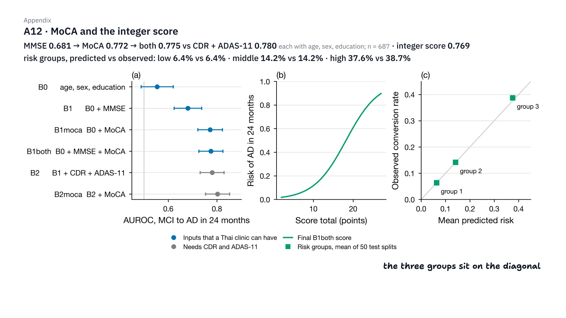
This is the detail of step 3. In 687 people, switching from MMSE to MoCA raises AUROC from 0.681 to 0.772; using both together gets 0.775, close to CDR + ADAS-11, which gets 0.780. The integer score gets 0.769. And when patients are split into 3 risk groups, the risk the table predicts and the real rate match: 6.4 and 6.4%, 14.2 and 14.2%, and 37.6 and 38.7%. So all three points sit right on the diagonal (near it, to be exact: the largest gap is 1.1 percentage points). If you want to see the full table, it’s in the “For doctors” section above.
Is sending MRI first to the people the model is unsure about better than random?
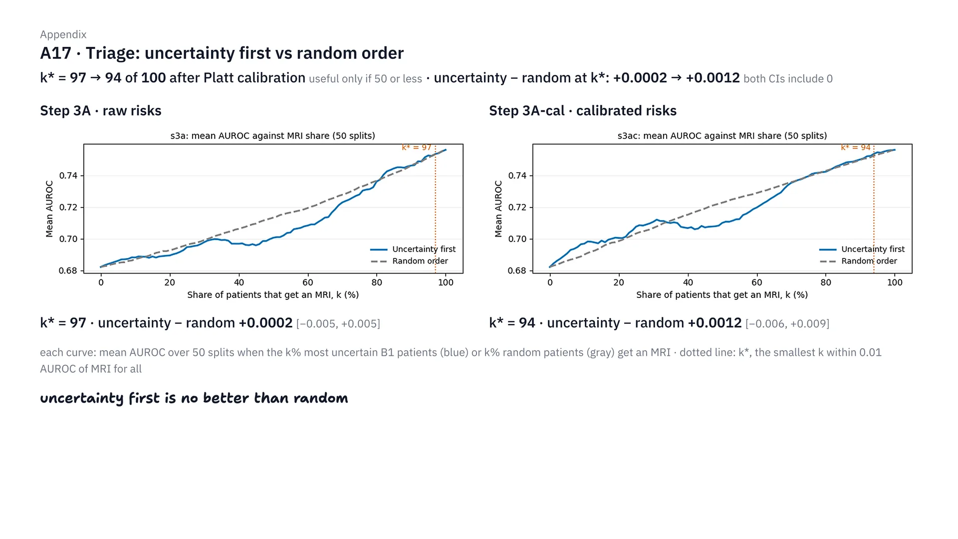
This figure compares two ways of choosing who to send for MRI. The first sends the people B1 is least sure about first; the second picks at random. Before and after calibration, you have to send 97 and then 94 of 100 people for scans, far over the 50 we set as the criterion. And at that point, choosing the unsure people first is no better than random at all: the differences are only +0.0002 and +0.0012, and the interval covers 0 in both. That’s why we shelved the triage plan.
Comparison with the source papers
What does the paper's basic set get on our data?
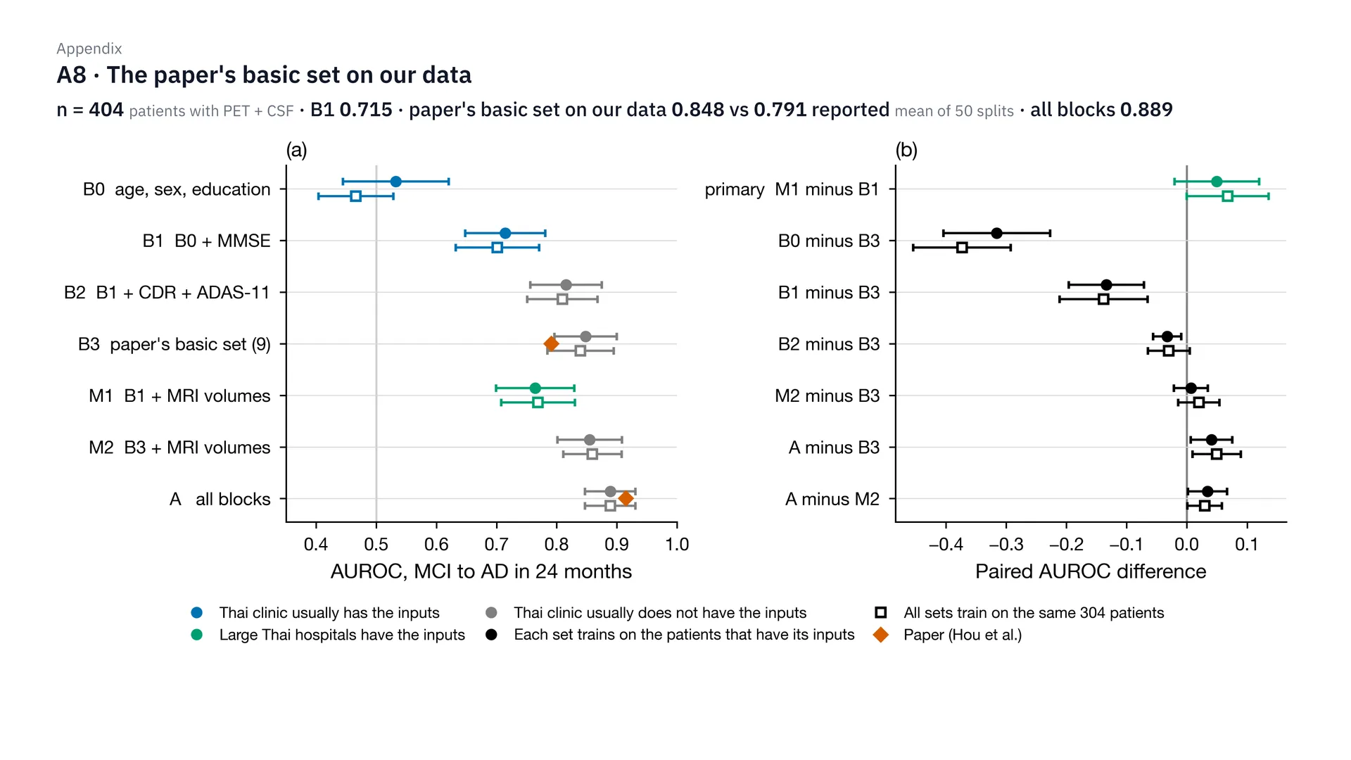
This is the first round, in 404 people with PET and CSF. The paper’s basic set, run on our data for 50 rounds, gets 0.848, which is even higher than the 0.791 the paper reported. The Thai basic set, B1, gets 0.715, and putting in everything, including PET and CSF, gets 0.889. Put simply, the paper’s basic isn’t basic for Thai clinics, because it has CDR, ADAS-11 and the APOE gene, which our clinics don’t have.
Why not deep learning?
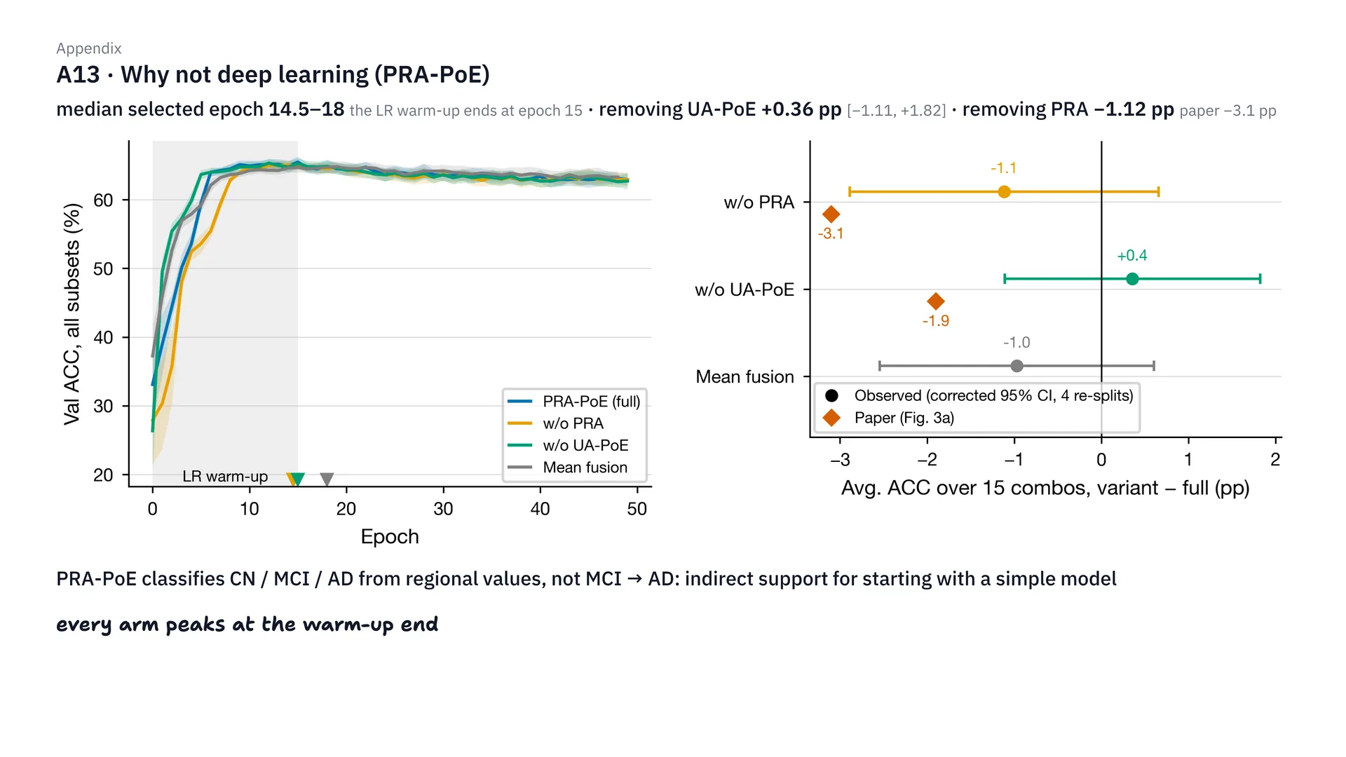
There’s a reason we don’t use deep learning, as follows. When replicating PRA-PoE, the best epoch was around 14.5–18, which is right where the learning rate warm-up ends, at epoch 15. That means after that, the model didn’t get any better at all. And removing UA-PoE didn’t make it worse — a difference of just +0.36 pp — while removing PRA made it worse by −1.12 pp, about a third of the −3.1 pp in the paper. But I should also say that PRA-PoE is a task of separating CN, MCI and AD, not directly our MCI-to-AD task, so this is indirect evidence.
Replicating Hou's paper: how did it turn out?
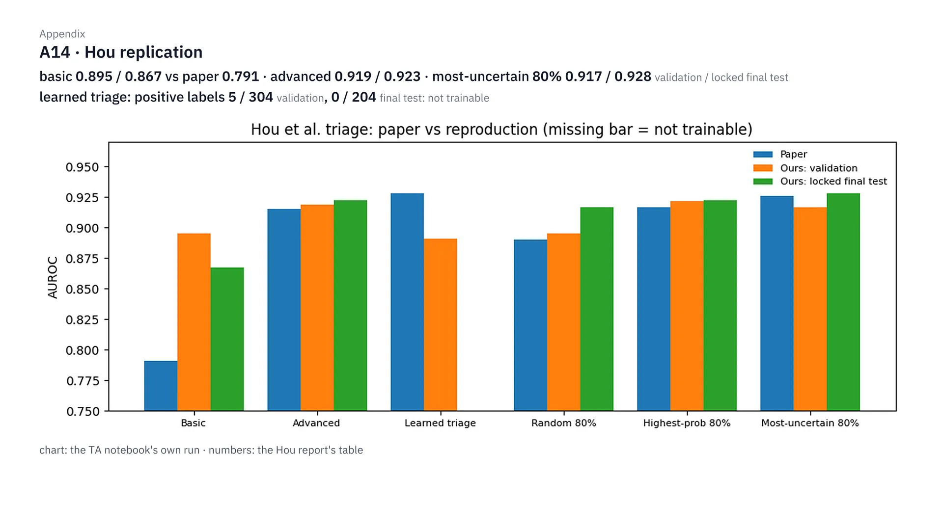
This is the result of replicating Hou’s paper. Our basic model is much stronger than the paper’s: 0.895 and 0.867, compared with the paper’s 0.791. Sending the 80% we’re least sure about to the advanced model gets 0.917 and 0.928, close to using the advanced model alone. But the learned triage, the paper’s highlight, doesn’t work on our data, because the labels used to train it have almost no positive cases: 5 of 304 people, and 0 of 204 people in the final test. As for the numbers swinging when you use a single test set, you can see it in how validation and the final test differ.
Inside PRA-PoE: how far can the modalities the model fills in be trusted?
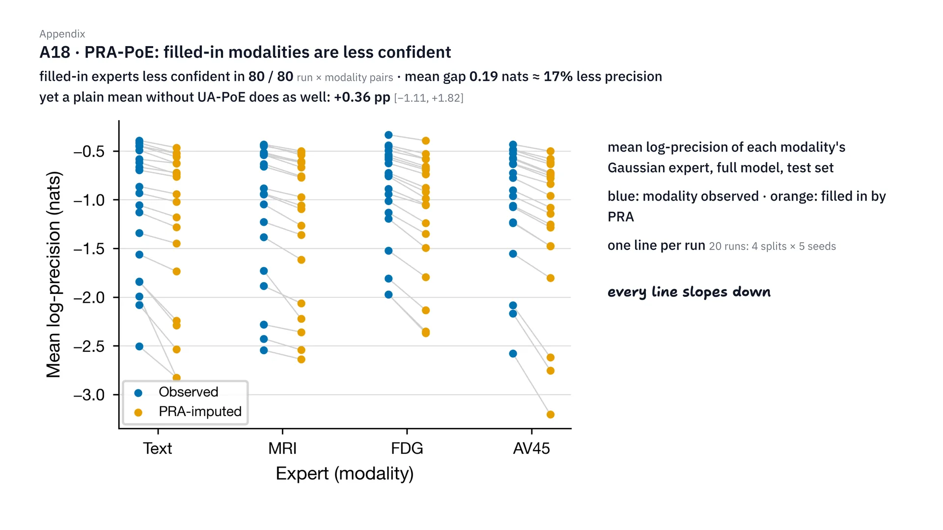
This one looks inside PRA-PoE. The modalities PRA fills in have less confidence than the real ones in every pair, 80 of 80 pairs, but the difference is only 0.19 nats, or about 17% less precision (precision here is the Gaussian expert’s inverse variance, not classification accuracy). So weighting them with UA-PoE doesn’t help, because a plain average gets about the same result, a difference of just +0.36 pp.
Does changing PRA-PoE's settings change the results?
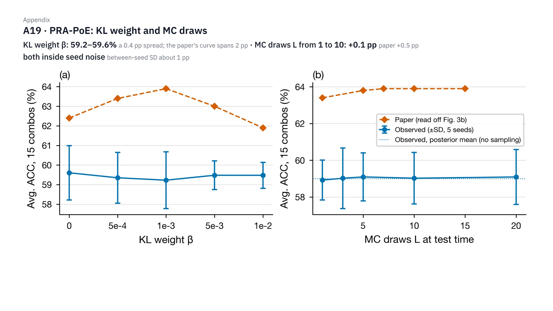
This is the sensitivity of PRA-PoE. Changing the KL weight β, accuracy stays at 59.2 to 59.6%, only 0.4 pp apart, while in the paper they’re as much as 2 pp apart. And raising the number of MC draws from 1 to 10 improves it by only 0.1 pp, compared with 0.5 pp in the paper. Both are within the noise level of changing the seed, which already swings about 1 pp. So we can conclude that these settings don’t affect our data.
Behind the scenes
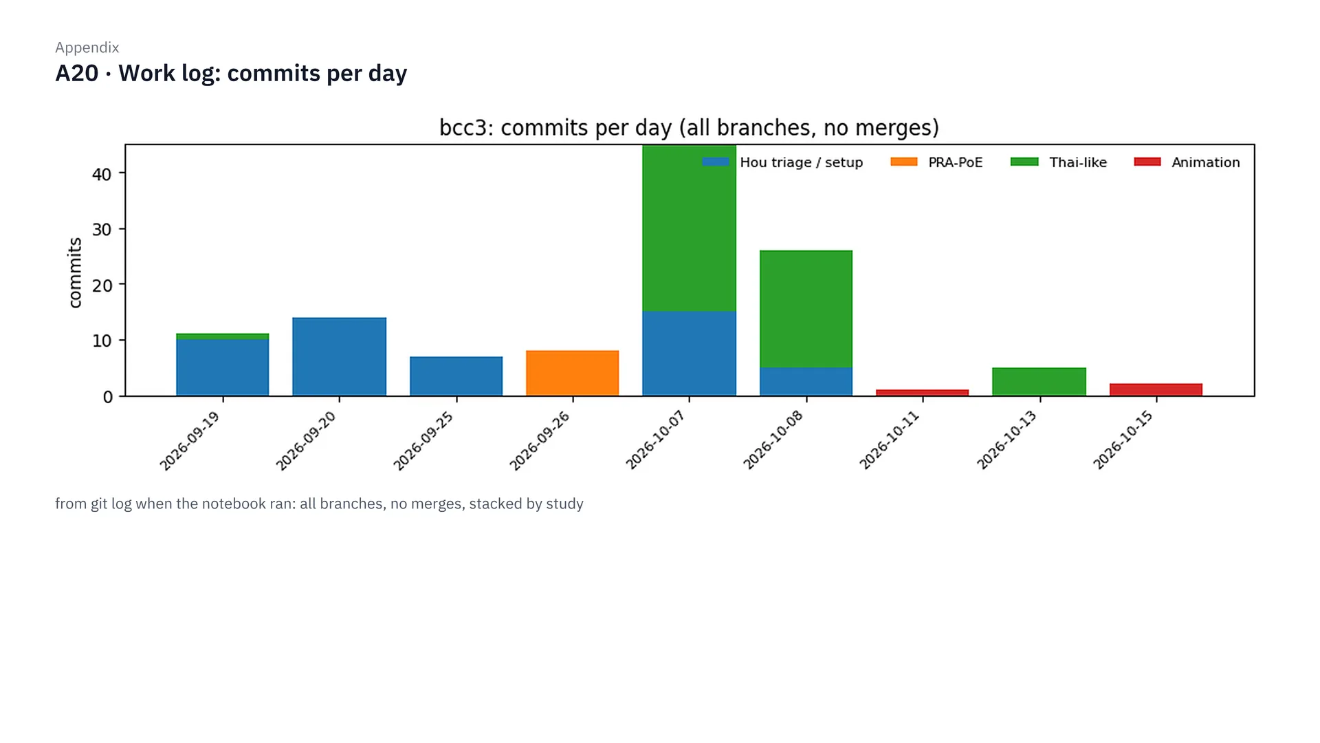
This figure is the work log: the number of commits per day, coloured by study, to show how this project went on step by step, from replicating the papers through each stage of the experiments.
References
- [1] Thaipisuttikul P, Jaikla K, Satthong S, Wisajun P. Rate of conversion from mild cognitive impairment to dementia in a Thai hospital-based population: A retrospective cohort. Alzheimers Dement (N Y). 2022. https://pmc.ncbi.nlm.nih.gov/articles/PMC8970424/
- [2] Hou, Tang, Jin. An Adaptive Machine Learning Triage Framework for Predicting Alzheimer’s Disease Progression. ML4H 2025 Findings. arXiv:2511.06681. https://arxiv.org/abs/2511.06681
- [3] Yang et al. PRA-PoE: Robust Multimodal Alzheimer’s Diagnosis with Arbitrary Missing Modalities. MICCAI 2026. arXiv:2605.13081. https://arxiv.org/abs/2605.13081
- [4] Sullivan LM, Massaro JM, D’Agostino RB Sr. Presentation of multivariate data for clinical use: The Framingham Study risk score functions. Stat Med. 2004;23(10):1631–60. doi:10.1002/sim.1742
- [5] Stern Y. Cognitive reserve in ageing and Alzheimer’s disease. Lancet Neurol. 2012;11(11):1006–12. doi:10.1016/S1474-4422(12)70191-6
- [6] Alzheimer’s Disease Neuroimaging Initiative (ADNI). adni.loni.usc.edu
Data from ADNI
The data used in this project come from ADNIMERGE2 0.1.1 (snapshot 2025-11-12) and from files downloaded from ADNI on 19 September 2026. This post shows only summary values; it contains no individual-level data.
Data used in preparation of this article were obtained from the Alzheimer’s Disease Neuroimaging Initiative (ADNI) database (adni.loni.usc.edu). As such, the investigators within the ADNI contributed to the design and implementation of ADNI and/or provided data but did not participate in analysis or writing of this report. A complete listing of ADNI investigators can be found at: http://adni.loni.usc.edu/wp-content/uploads/how_to_apply/ADNI_Acknowledgement_List.pdf
The ADNI was launched in 2003 as a public-private partnership, led by Principal Investigator Michael W. Weiner, MD. The original goal of ADNI was to test whether serial magnetic resonance imaging (MRI), positron emission tomography (PET), other biological markers, and clinical and neuropsychological assessment can be combined to measure the progression of mild cognitive impairment (MCI) and early Alzheimer’s disease (AD). The current goals include validating biomarkers for clinical trials, improving the generalizability of ADNI data by increasing diversity in the participant cohort, and to provide data concerning the diagnosis and progression of Alzheimer’s disease to the scientific community. For up-to-date information, see adni.loni.usc.edu.
Data collection and sharing for the Alzheimer’s Disease Neuroimaging Initiative (ADNI) is funded by the National Institute on Aging (National Institutes of Health Grant U19AG024904). The grantee organization is the Northern California Institute for Research and Education. In the past, ADNI has also received funding from the National Institute of Biomedical Imaging and Bioengineering, the Canadian Institutes of Health Research, and private sector contributions through the Foundation for the National Institutes of Health (FNIH) including generous contributions from the following: AbbVie, Alzheimer’s Association; Alzheimer’s Drug Discovery Foundation; Araclon Biotech; BioClinica, Inc.; Biogen; Bristol-Myers Squibb Company; CereSpir, Inc.; Cogstate; Eisai Inc.; Elan Pharmaceuticals, Inc.; Eli Lilly and Company; EuroImmun; F. Hoffmann-La Roche Ltd and its affiliated company Genentech, Inc.; Fujirebio; GE Healthcare; IXICO Ltd.; Janssen Alzheimer Immunotherapy Research & Development, LLC.; Johnson & Johnson Pharmaceutical Research & Development LLC.; Lumosity; Lundbeck; Merck & Co., Inc.; Meso Scale Diagnostics, LLC.; NeuroRx Research; Neurotrack Technologies; Novartis Pharmaceuticals Corporation; Pfizer Inc.; Piramal Imaging; Servier; Takeda Pharmaceutical Company; and Transition Therapeutics.
ทำนาย MCI สู่อัลไซเมอร์ ด้วยข้อมูลที่คลินิกไทยมีจริง
สรุปสั้นๆ
- คำถาม: ถ้าตัดการตรวจราคาแพงอย่าง PET scan, CSF และยีน APOE ออก เรายังทำนายได้ไหมว่าผู้ป่วย MCI คนไหนจะเป็นอัลไซเมอร์ภายใน 24 เดือน (นานสุด 30 เดือนเมื่อรวมช่วงเผื่อของวันนัดตรวจ)
- “เป็นอัลไซเมอร์” ในงานนี้หมายถึง ADNI วินิจฉัยว่าเป็นภาวะสมองเสื่อม (dementia) ภายใน 30 เดือนนับจากวันแรกที่เป็น MCI (เป้า 24 เดือน บวกช่วงเผื่อ 6 เดือน) ไม่ใช่พยาธิสภาพอัลไซเมอร์ที่ยืนยันด้วย biomarker และคนที่ไม่ convert แต่ติดตามไม่ถึง 18 เดือนถูกตัดออก ตัวเลข 25.5% ที่ convert จึงไม่ใช่อัตราการเปลี่ยนของ MCI ทั่วไป
- สำหรับโรงพยาบาลที่มี MRI: ชุด 4 ตัวแปร (อายุ ปีการศึกษา MoCA และ hippocampal volume คู่กับ ICV) ได้ AUROC 0.815
- สำหรับคลินิกที่ไม่มี MRI: ตารางคะแนนบนกระดาษที่ใช้ MoCA, MMSE, เพศ และปีการศึกษา ได้ AUROC ประมาณ 0.769
- คุณหมอที่อยากลองใช้ตารางคะแนนนี้: วิธีใช้ทีละขั้น ตารางเต็ม และข้อจำกัด อยู่ในหัวข้อ “สำหรับคุณหมอ” ด้านล่าง
- ทั้งหมดเป็นงานวิจัยบนข้อมูล ADNI ยังไม่ได้ validate กับคนไข้ไทย ห้ามใช้ตัดสินการวินิจฉัยหรือการรักษา
ที่มา: อัลไซเมอร์กับข้อจำกัดของคลินิกไทย
ในประเทศไทย การเข้าถึง modality ในการวินิจฉัยโรคต่างๆ อาจจะไม่ได้มีในทุกโรงพยาบาล แล้วก็อาจจะมีคนอีกจำนวนหนึ่งเลยที่อาจจะไม่ได้มีกำลังทรัพย์ หรือความสามารถในการที่จะเข้าถึง modality เหล่านั้นได้ด้วยซ้ำ ซึ่งหนึ่งในระบบที่ต้องใช้ modality ในการวินิจฉัยเยอะก็คือโรคทางระบบประสาท และหนึ่งในภาวะที่เจอเยอะมากในโรคระบบประสาทก็คือภาวะอัลไซเมอร์ครับ
ภาวะอัลไซเมอร์มีประเด็นหนึ่งที่ผมว่าค่อนข้างน่าสนใจ ก็คือภาวะการ progression จากภาวะ mild cognitive impairment หรือ MCI ไปสู่ Alzheimer’s disease หรือ AD จากงานวิจัยของโรงพยาบาลรามาธิบดี[1] พบว่าจากผู้ป่วยประมาณ 250 คน จะมีการพัฒนาจาก MCI ไปเป็น AD (งานวิจัยนี้นับการเปลี่ยนเป็นภาวะสมองเสื่อม ไม่ได้นับเฉพาะอัลไซเมอร์) ภายใน 1 ปีถึง 18.4% คือประมาณหนึ่งในห้าเลย ซึ่งการที่เราบอกได้ว่าคนไหนจะพัฒนาจาก MCI ไปเป็น AD ก็จะทำให้แพทย์สามารถวางแผนการรักษาได้ดีขึ้น จริงไหมครับ
แต่การที่เราจะทำให้โมเดลทำนายภาวะ progression ตรงนี้ได้อย่างแม่นยำ ในงานวิจัยต่างประเทศส่วนใหญ่ เราก็จะต้องใช้ modality ที่มีราคาแพง หรือเป็น invasive diagnosis ไม่ว่าจะเป็นการทำ PET scan, CSF หรือการตรวจหายีน APOE ซึ่งหลายๆ โรงพยาบาลในไทยก็ยังมีข้อจำกัดในการเข้าถึง modality เหล่านี้
ซึ่งมันก็คงจะดีมากๆ เลยใช่ไหมครับ ถ้าเราสามารถตัด modality แพงๆ หรือ invasive diagnosis ต่างๆ ออกไป แต่เราก็ยังจะสามารถทำนายภาวะ progression จาก MCI ไปเป็น AD ได้อย่างแม่นยำเหมือนเดิม คำถามก็คือ แล้วเราทำได้ไหม และถ้ามันทำได้ เราจะต้องอาศัย feature อะไรบ้าง หรือพูดง่ายๆ ก็คือ เราต้องใช้ข้อมูลอะไรบ้างในการ prediction ของโมเดล และนี่ก็คือที่มาของ project ที่ผมทำใน Brain Code Camp 2026 ครับ
ภาพรวม: จากข้อมูลสู่ชุดเครื่องมือ
ทีนี้เรามาดูภาพรวมของ project ก่อนแล้วกัน ก็คือ มันเริ่มต้นจากเราต้องการเลือก dataset ใช่ไหมครับว่า โอเค เราจะใช้ dataset อะไรในการทำ project นี้ แล้วก็เนื่องจากประเทศไทยไม่ได้มีตัว public dataset ออกมาเยอะมาก หรือไม่ได้มี public dataset ออกมาในเชิงที่เราจะใช้ในการ train model เพื่อดู progression จาก MCI ไปเป็น Alzheimer’s ใช่ไหม เราก็เลยใช้ตัว ADNI dataset[6] มาใช้แทน ซึ่ง ADNI ก็คือข้อมูลผู้ป่วยอัลไซเมอร์ใน North America พอเราได้ข้อมูลมาเสร็จปุ๊บ เราก็เอาข้อมูลมาทำ EDA แล้วก็ cleansing data ไม่ว่าจะเป็นการคัดกรองคนไข้ แก้ไขเรื่องอายุต่างๆ เดี๋ยวผมจะพูดรายละเอียดพวกนี้ทีหลัง แล้วก็มีการ merge ในฝั่ง tabular data ของ MRI ต่างๆ มีการ calculate ตัว MoCA score ใหม่ ทั้งหมดนี้เป็นการเตรียมความพร้อมของ dataset ที่เราจะเอาไปใช้ในการ train model ได้ออกมาเป็นผู้ป่วยที่เป็น MCI ทั้งหมด 1,063 คนครับ
แล้วเราก็ทำการ pre-processing โดยป้องกัน data leakage หมายถึงว่าไม่ให้มันมี bias โดยการแยกชุด train กับ test ออกชัดเจน แล้วเราก็ทำการ scope เฉพาะสิ่งที่ประเทศไทยมี ผมก็เลย label มันว่าเป็น Thai-like data นั่นก็คือพวกอายุ เพศ ปีการศึกษา MMSE แล้วก็ MoCA score แล้วก็ใส่ตัว T1W MRI ซึ่งจะมีสองค่าก็คือ hippocampal volume กับ ICV ครับ ซึ่ง T1W ที่ผมใช้ เขาจะคำนวณโดยใช้โปรแกรม FreeSurfer แล้ววัดปริมาตรออกมาเป็นตัวเลขในตาราง ค่าที่เราใช้ก็คือ hippocampal volume แล้วก็ ICV ก็คือ intracranial volume ครับ
ขอขยายนิดนึงว่าจากภาพสแกนมันกลายเป็นตัวเลขได้ยังไง ภาพ T1 MRI เป็นภาพสามมิติ เหมือนขนมปังทั้งก้อนที่หั่นเป็นแผ่นบางๆ แต่ละแผ่นประกอบด้วยลูกบาศก์จิ๋วขนาดประมาณ 1 มิลลิเมตรที่เรียกว่า voxel โปรแกรม FreeSurfer จะระบายสีให้อัตโนมัติว่า voxel ไหนเป็นสมองส่วนไหน แล้วนับ voxel ที่เป็น hippocampus ทั้งซีกซ้ายและซีกขวา ออกมาเป็นปริมาตรหน่วยลูกบาศก์มิลลิเมตรครับ ADNI เขาทำขั้นตอนนี้มาให้แล้ว เราเอาตารางที่ได้มาใช้ต่อเลย
ถ้าดูภาพประกอบทีละขั้น เริ่มต้นจาก ขั้นที่ 1 ภาพ T1 MRI เป็นภาพสามมิติที่ประกอบด้วยลูกบาศก์จิ๋วขนาดประมาณ 1 มิลลิเมตรที่เรียกว่า voxel จากนั้นใน ขั้นที่ 2 โปรแกรม FreeSurfer จะระบายสีให้อัตโนมัติว่า voxel ไหนเป็น hippocampus ซีกซ้าย ซีกขวา แล้วก็ตีกรอบโพรงกะโหลกที่เรียกว่า ICV พอระบายสีเสร็จ ใน ขั้นที่ 3 ก็นับ voxel ของ hippocampus สองข้างรวมกัน ออกมาเป็นปริมาตรหน่วยลูกบาศก์มิลลิเมตร และใน ขั้นที่ 4 ที่เราต้องใส่ ICV คู่กันเสมอ ก็เพราะคนหัวใหญ่ก็มีสมองใหญ่อยู่แล้ว ICV ช่วยให้โมเดลแยกได้ว่า hippocampus ที่เล็ก เล็กเพราะฝ่อจริงๆ หรือเพราะหัวเล็ก ซึ่งตัวเลขพวกนี้ ADNI เขาทำมาให้แล้ว ส่วนโรงพยาบาลไทยจะได้ค่านี้มาจากไหน ก็เป็นข้อจำกัดข้อแรกที่ผมพูดไว้ในหัวข้อข้อจำกัดด้านล่างครับ
ทีนี้ในขั้นตอนการทำ model development เราก็ไปดูว่ามันมี paper ไหนที่ทำคล้ายๆ เรา หมายถึงว่าการตัด modality ออก โดยเฉพาะที่เขาโฟกัสที่ตัว ADNI dataset เราก็เลยเจอ paper สองอัน ก็คือปี 2025 ของ Hou et al.[2] กับปี 2026 ของ PRA-PoE[3] แล้วสุดท้ายเราก็เลือกใช้ตัว penalized logistic regression โดยใช้ 50 paired splits เดี๋ยวเล่ารายละเอียดในหัวข้อถัดไป แล้วเราก็ไปทำ development ตัว experiment บน Thai-like data
แล้วสุดท้าย ส่วน Output เราก็จะได้ชุดตัวเลือกหรือ candidate ในสองบริบท ก็คือบริบทที่มี MRI กับไม่มี MRI ซึ่งเดี๋ยวผมเล่าต่อด้านล่างครับ
เรียนอะไรจาก 2 papers ต้นแบบ
ก่อนที่เราจะไปเริ่มดู data cleansing ผมขอเล่าให้ฟังสั้นๆ ว่าทำไมเราถึง train โมเดลในลักษณะแบบนี้ คือตอนแรก วัตถุประสงค์ของ project เราก็คือเราอยากลองตัด modality ราคาแพงออกใช่ไหมฮะ ซึ่งเราก็เลยลองไปดูว่ามันมี paper อะไรที่ใกล้เคียงกับของเราบ้าง แล้วก็เลยไปเจอ paper ของ Hou ปี 2025 เขาทำเรื่อง adaptive triage ก็คือเอาโมเดลพื้นฐานมาทำการคัดกรองคนไข้ ก่อนที่จะส่งเขาไปตรวจแบบราคาแพงต่อไป แล้วก็มีอีก paper หนึ่งของ Yang ที่เขาทำเรื่อง PRA-PoE ก็คือลองเอาตัว deep learning model มาช่วย predict คนไข้ที่ตรวจ modality ไม่ครบ
ผมก็เลยลองเอาสอง paper มาลอง replicate กับตัว ADNI dataset ที่ผมมีจริงๆ แล้วก็ลองทำตามวิธีของเขา อันแรกที่ผมเจอเลยก็คือ คำว่า cheap หรือ cheap basic data ใน paper ของเขา มันไม่ได้แปลความเหมือนกับว่ามันเป็น cheap จริงๆ ในประเทศเรา หมายถึงว่าเขามีการใส่ตัว CDR ก็คือ Clinical Dementia Rating ซึ่งในประเทศเราไม่ได้มีการทำพวกนี้ หรือตัว ADAS-11 พวกเนี้ยเราก็ไม่ได้ทำ แล้วก็พวกยีน APOE ก็รวมเข้าไปอยู่ใน cheap ของเขาด้วย แต่ในขณะที่โรงพยาบาลในไทย สิ่งพวกเนี้ยเราไม่ได้ตรวจเป็นประจำ เพราะงั้นถ้าเราจะจัดเป็น feature ของข้อมูล เราก็ควรจะจัดให้มันล้อไปกับความจริงของประเทศไทยด้วย
อันที่สองก็คือ พอเราเริ่มทดลอง replicate paper ของ Yang กับ dataset ของเรา เราก็เลยเห็นว่าตัว deep learning model ที่เราทำ มันมีการ overfitting ที่ epoch ประมาณ 15–18 คือความแม่นยำของชุด validation ขึ้นไปสูงสุดประมาณตรงช่วง epoch นั้น ซึ่งพอเรา train ต่อไป มันก็จะไม่ได้ดีขึ้นแล้ว เพราะว่าข้อมูลของเรามันมีแค่ประมาณหลักร้อยหลักพัน (ย้อนดูแล้ว จุดสูงสุดนี้ตรงกับตอนที่ learning-rate warm-up จบที่ epoch 15 พอดี จึงเป็นหลักฐานทางอ้อมให้เลือกโมเดลที่ง่ายกว่า ไม่ได้พิสูจน์ว่าโมเดล overfit จริง และไม่ได้พิสูจน์ว่าข้อมูลน้อยเป็นสาเหตุ) ซึ่งอันนี้แหละก็คือปัญหาของการ overfitting ผมก็เลยตัดสินใจว่า โอเค deep learning อาจจะไม่ได้เหมาะกับเราเท่าไหร่ ผมก็เลยตัดในส่วนของ deep learning ไม่ได้ไปต่อตรงนี้ เพราะมันไม่ได้ช่วยบนข้อมูลชุดนี้เท่าไหร่
สุดท้ายเราก็เลยตัดสินใจว่า โอเค เรามาทำตัว interpretable linear model ดีกว่า หรือพูดง่ายๆ ก็คือ เราก็ใช้ตัว linear model แล้วเราก็เปิดดู weight ข้างในได้ครับว่า feature อันไหนมันมีความสำคัญมากน้อยเป็นยังไง หมายถึงว่า weight มันเป็นยังไง ซึ่งมันก็คือสูตรของ Hou นั่นแหละครับ แล้วเราก็ทำ penalized logistic regression มาเป็นโมเดลหลัก ซึ่งคำว่า penalized logistic regression ก็คือ เหมือนเราทำ logistic regression แต่เราใส่ตัว L2 regularization เข้าไป เพื่อช่วยกดไม่ให้โมเดลเทน้ำหนักไปที่ค่าใดค่าหนึ่งมากเกินไป ก็เพราะว่าเราไม่ได้อยากให้มันไป overfitting แล้วก็ส่วนของค่า C เราก็กำหนดว่า พวกที่เป็น basic information ต่างๆ เราจะตั้งไว้ที่ 0.1 เพราะชุดนี้มีตัวแปรไม่กี่ตัว แล้วก็เราจะให้ค่า C เป็น 0.01 กับข้อมูลพวก MRI อะไรอย่างเงี้ย เพราะว่าข้อมูลสมองมันมีตัวแปรเยอะและสัมพันธ์กันสูง เราก็ไม่ได้อยากให้โมเดลมันไป overfitting กับตรงนั้นมากจนเกินไปครับ
สุดท้ายก็คือเรื่องที่สาม ก็คือ paper ของ Hou เขาวัดผลบน test set ชุดเดียว 100 คน ซึ่งพอเราสุ่มใหม่แล้วตัวเลขมันมีความแกว่งมากๆ เราก็เลยทำ evaluation ด้วยการทำ paired splits 50 คู่ คือสุ่มแบ่งข้อมูลชุด train กับ test ออกมา 50 รอบ เพื่อให้ตัวเลขไม่ขึ้นกับดวงของการสุ่มแค่รอบเดียวครับ
เตรียมข้อมูล: คัดคนไข้ แก้บั๊ก และกัน data leakage
พอเราวางกรอบการทดลอง settled แล้ว เราก็มาทำ EDA กับ cleaning data ของ ADNI ที่เราดาวน์โหลดมา ซึ่งก็จะประกอบไปด้วย 3 ส่วน
ส่วนแรก เราทำ cohort filtering ก็คือหมายถึงว่า ข้อมูลมันมี 3,700 กว่าคนใช่ปะครับ เราตัดคนที่ไม่ใช่ MCI ออก แล้วก็คนที่ไม่เปลี่ยนเป็น AD แต่ติดตามไม่ถึง 18 เดือนออก เพื่อไม่ให้คนที่หายไปกลางคันมาปน สุดท้ายเราก็จะเหลือผู้ป่วย MCI ที่เราจะเอาเข้ากลุ่มมาอยู่ที่ 1,063 คน แล้วก็ในกลุ่มนี้ก็จะเปลี่ยนไปเป็น AD ทั้งหมด 271 คน หรือคิดเป็น 25.5% ซึ่งก็ตรงกับตัวเลขทางสถิติครับ
ส่วนที่สองก็คือเราทำ data audit ซึ่งเราเจอปัญหา 3 อัน อันแรกก็คือเรื่องอายุ เนื่องจากตัว ADNI dataset มันบันทึกอายุตอนที่สมัครครั้งแรก (ที่ถูกคืออายุ baseline ของเฟส ADNI ปัจจุบัน) ไม่ใช่ตอนที่เริ่ม develop เป็น MCI ซึ่งบางคนก็จะมีค่าที่ผิดเพี้ยนค่อนข้างเยอะ เราก็เลยคำนวณใหม่
อันที่สองก็คือตาราง tabular ของ MRI ซึ่งตัวนี้มันก็คือการที่เขาเอาภาพ MRI ไปเข้า FreeSurfer แล้วก็แปลงเป็นตารางเข้ามาอยู่ใน ADNI dataset ซึ่งมันจะมี 2 เวอร์ชัน อันแรกเป็น FreeSurfer 5.1 ปรากฏว่าความครบของข้อมูลมันอยู่แค่ 40.3% ในขณะที่ FreeSurfer version 6.0 มันจะมีอยู่ที่ 17.1% เราก็เลยจับสองตารางนี้มา merge กัน แล้วก็จับคู่ผลสแกนต่างๆ ครับ ก็เลยได้ความครบถ้วนอยู่ที่ 57.4% พูดง่ายๆ ก็คือประมาณ 610 คน (57.4% คือสัดส่วนที่จับคู่วันสแกนได้ ส่วนคนที่มีปริมาตรครบจริงคือ 578 คน) พร้อมกับเอาผลสแกนวันเดียวกันที่ซ้ำ 538 คู่ มาหาค่าเฉลี่ย แล้วก็มาคัดคนที่ข้อมูลสมองครบถ้วน เราก็จะได้กลุ่ม MRI test 568 คน แล้วก็จะมีกลุ่มที่มีทั้ง MoCA แล้วก็ตัว hippocampus อยู่ที่ 574 คนครับ
สุดท้ายก็คือตัว MoCA score ครับ ในตารางของ ADNI คนไข้ที่ตรวจในเฟสใหม่ๆ เขาจะมีคอลัมน์ที่รวมคะแนนเต็ม 30 มาให้แล้ว แต่มีคนไข้แค่ 230 คนครับ ส่วนคนไข้ในเฟสเก่าๆ คอลัมน์คะแนนรวมมันยังไม่ได้รวมมาให้ เราก็เลยลองเข้าไป explore ดูใน ADNI database แล้วก็ค้นพบว่าเขาเก็บผลตรงเนี้ยแยกเป็นรายข้อไว้ให้ครบทั้ง 30 คอลัมน์ (ที่ถูกคือ 32 คอลัมน์ที่ให้คะแนน รวมเป็นเต็ม 30) เช่น สมมติว่าข้อวาดรูปนาฬิกาได้ไหม อะไรเงี้ย หรือลบเลขทีละ 7 อะไรแบบเนี้ยครับ เราเลย recalculate ใหม่ ก็คือเขียนสูตรเข้าไปคำนวณคนไข้เฟสใหม่ที่มีคะแนนรวมอยู่แล้วก่อน แล้วก็พบว่า อ๋อ โอเค มันถูกต้องแล้ว พอสูตรนี้ถูกต้อง เราก็เลยเอาไป convert คนไข้เฟสเก่าให้ขึ้นมาด้วย ก็เลยได้ทั้งหมด 687 คนครับผม ที่ทั้ง recalculate แล้วก็ revalidate แล้ว
และส่วนสุดท้าย ก็คือการป้องกัน data leakage ครับ data leakage ก็คือการที่ข้อมูลของชุด test แอบรั่วเข้าไปตอนเรา train โมเดล ซึ่งจะทำให้ผลออกมาดีเกินจริง เหมือนนักเรียนได้เห็นข้อสอบก่อนสอบ เราเลยป้องกันแบบนี้ครับ ในทุกรอบของ 50 splits พอเราแบ่งชุด train กับ test แล้ว ตัวเลขที่ใช้เตรียมข้อมูล ไม่ว่าจะเป็นค่า median ที่ใช้เติมช่องที่ข้อมูลหาย หรือค่า mean กับ SD ที่ใช้ปรับสเกลแบบ Z-score เราจะคำนวณจากคนในชุด train เท่านั้น แล้วค่อยเอาตัวเลขชุดเดียวกันนี้ไปใช้กับชุด test ครับ ชุด test ก็เลยเหมือนคนไข้ใหม่ที่โมเดลไม่เคยเห็นจริงๆ
เลือก feature ให้ตรงกับคลินิกไทย
ทีนี้พอเราคลีนข้อมูล settled แล้วใช่ไหมครับ สเต็ปถัดมาเราก็มาทำการเลือก feature ให้ตรงกับบริบทของโรงพยาบาลในไทย เพื่อเอาไป train model ต่อครับ
เราอ้างอิงจากงานวิจัยของโรงพยาบาลรามาของผู้ป่วย MCI 250 คนที่ผมกล่าวไปข้างต้น ทำให้เราแบ่ง feature ของไทยเป็น 2 ระดับ ก็คือระดับแรกคือข้อมูลพื้นฐานจริงๆ ที่แทบทุกโรงพยาบาลเก็บอยู่แล้ว ก็คือพวกอายุ เพศ การศึกษา แล้วก็คะแนน MMSE ซึ่งจริงๆ เดี๋ยวในขั้นที่ 4 เราจะดูกันว่าอันไหนที่โมเดลจะให้ AUC สูงสุด
AUC หรือชื่อเต็มๆ ว่า AUROC ให้นึกถึงเกมทายคู่ครับ หยิบคนไข้มาคู่นึง คนหนึ่งจะ progress เป็น AD อีกคนหนึ่งไม่เป็น แล้วให้โมเดลชี้ว่าใครเสี่ยงกว่า AUROC ก็คือโมเดลชี้ถูกบ่อยแค่ไหนจากทุกคู่ ถ้าได้ 0.5 ก็เท่ากับโยนเหรียญ ถ้าได้ 1 ก็คือชี้ถูกทุกคู่ ยิ่งเข้าใกล้ 1 ยิ่งดีครับ
แต่ตอนเนี้ยเรารวมพวกนี้เข้าไปก่อน โดยที่เราตั้งชื่อชุดข้อมูลพื้นฐานทางคลินิกอันเนี้ยครับว่า B1 ละกัน เพื่อความง่าย ส่วนระดับที่สอง คือสิ่งที่โรงพยาบาลไทยสามารถตรวจเพิ่มได้ในผู้ป่วยประมาณครึ่งหนึ่ง ก็คือพวกการทำ MoCA score กับการทำ MRI โดยที่โฟกัสไปที่ T1-weighted MRI ก่อน ส่วนแบบประเมินที่ใช้เวลานาน แล้วก็รวมไปถึงพวก PET scan หรือการเจาะ CSF หรือการตรวจยีนพวก APOE อะไรแบบเนี้ยครับ ที่ไม่ได้มีใน cohort ที่อ้างอิงของโรงพยาบาลรามา เราก็เลยเลือกที่จะไม่ใช้ในการ train model
ส่วนวิธีการ train model ก็อย่างที่เราเล่าไป ก็คือเราใช้ penalized logistic regression โดยใส่ class weight ให้เป็น balanced เพื่อตัดปัญหาเรื่อง class ที่มันไม่สมดุล แล้วเราก็ใช้ L2 regularization ตามสูตรของ paper ของ Hou ปี 2025 เลย ก็คือให้ C เท่ากับ 0.1 สำหรับข้อมูลทางคลินิก แล้วก็ให้ค่า C เท่ากับ 0.01 สำหรับข้อมูลที่เป็นกลุ่มพวก MRI ในขั้นทดสอบการแยกโมดูล ส่วนในขั้นสุดท้ายที่เราเปรียบเทียบ 63 รูปแบบ ที่ผมบอกว่าเราจะมีการเทียบทุกอัน เราก็เลยล็อกค่า C เท่ากับ 0.1 เท่ากันทุกชุดไปเลย เพื่อวัดผลของ feature ให้มันยุติธรรมที่สุดครับ
ขั้นที่ 1: ข้อมูลพื้นฐานพอไหม และ MRI ช่วยแค่ไหน
ทีนี้เรามาดูผลการทดลองขั้นแรกกัน ก็คือ ตอนแรกที่เรา run ตัว model ครับ เราใช้ข้อมูล B1 จาก n 404 คน ซึ่ง 404 คนก็คือเราคัดเลือกมาจากคนที่มีข้อมูล PET scan, CSF อะไรพวกเนี้ยครบ แล้วเราก็จะพบว่าถ้าเราใช้แค่ตัวข้อมูล age, sex แล้วก็ education คืออายุ เพศ และการศึกษาครับ จะได้ AUROC อยู่ที่แค่ประมาณ 0.53 เท่านั้น ซึ่งมันก็ประมาณโยนเหรียญนั่นเอง แต่พอเราลองเพิ่มตัว MMSE เข้าไป ซึ่ง MMSE ก็จะเป็นแบบทดสอบอันหนึ่ง จะทำให้ค่า AUROC กระโดดขึ้นมาเป็น 0.715 แต่ก็ยังต่ำกว่าชุด basic ของตัว paper ที่เราเอามารันกับข้อมูลของเราอยู่ดี ซึ่งได้อยู่ที่ประมาณ 0.848 ซึ่งจะเห็นว่ามันแตกต่างกันอยู่พอสมควร
แล้วก็ปัญหาที่เจอในการรันครั้งแรกอีกอันนึงก็คือ พอเราใส่ค่า MRI เข้าไป ที่เราคาดหวังว่าจะไปช่วยให้ค่า AUROC ขยับขึ้นมา มันก็ขยับขึ้นมาที่ 0.764 แต่ตัว confidence interval จะเห็นว่ามันมี range ที่ค่อนข้างกว้างเกินไป คือช่วงความต่างมันแกว่งตั้งแต่ติดลบไปจนถึงบวก ทำให้เรารู้สึกว่าข้อสรุปอันเนี้ยมันยังไม่ชัดเจนว่า การเพิ่ม MRI เข้าไป มันจะทำให้โมเดลแม่นยำขึ้นจริงหรือเปล่า
ทีนี้ผมก็เลยลองไปสังเกตดูอีกครั้ง แล้วก็ลองรันอีกรอบ แต่รอบนี้คือ สุดท้ายเราอาจจะไม่ได้สนใจตัว PET scan กับ CSF อยู่แล้วใช่ไหมครับ เพราะว่าในไทย มันไม่ได้เป็นการวินิจฉัยที่แพร่หลาย ไม่ได้เป็น modality ที่อยู่ใน feature ที่เราจะใส่อยู่แล้ว ผมก็เลยอยากเพิ่ม n โดยรอบที่สอง เราเอาเงื่อนไขของ PET scan กับ CSF ออก เราก็เลยจะได้ n มาเป็น 568 คน
แล้วเราก็ลองเทียบดูว่าต้องใช้ข้อมูล MRI มากแค่ไหนถึงจะพอ โดยลอง 3 แบบครับ คือแบบแรกเราใช้แค่ตัว hippocampus volume ซึ่งเป็นสมองส่วนความจำ คู่กับตัว ICV หรือปริมาตรภายในกะโหลก ที่เอาไว้ปรับให้เทียบกันได้ระหว่างคนหัวเล็กกับหัวใหญ่ แบบที่สองก็คือเราใช้ปริมาตร MRI 4 ค่าเลย คือเพิ่ม entorhinal cortex ซึ่งเป็นสมองส่วนที่อยู่ติดกับ hippocampus และเป็นจุดแรกๆ ที่อัลไซเมอร์เริ่มทำลาย กับ ventricles หรือโพรงน้ำในสมอง ที่จะขยายใหญ่ขึ้นเมื่อเนื้อสมองฝ่อ เข้าไปด้วย แล้วแบบที่สามก็คือดึงมาทั้ง 117 ส่วนทั่วสมองเลย พร้อมจูนค่า C ให้ด้วย ซึ่งค่า C ก็คือความแรงของการกดน้ำหนักโมเดลที่ผมเล่าไปตอนต้น (ที่ถูกคือกลับกัน ค่า C ยิ่งน้อย การกดยิ่งแรง) การจูนก็คือแทนที่จะล็อกค่าไว้ เราให้โมเดลลองหลายๆ ค่าในชุด train แล้วเลือกค่าที่เหมาะที่สุดเอง แล้วดูว่าแบบไหนเวิร์คที่สุด
ผลออกมาก็คือชัดเจนเลยครับว่า ในกลุ่ม 568 คน การเพิ่มแค่ตัว hippocampus กับตัว ICV จะดึงให้ตัว AUROC จาก 0.682 เพิ่มขึ้นไปเป็น 0.756 หรือพูดง่ายๆ คือเพิ่มถึง 0.074 เลย ชนะถึง 49 จาก 50 รอบเลย แล้วก็ให้ผลใกล้เคียงกับการใช้ 4 ส่วนหลักมากๆ ในขณะที่การใส่สมองทั้ง 117 ส่วน ไม่ได้เพิ่มความแม่นยำเหนือโมเดล 4 ส่วนหลักที่จูนค่า C แล้วอย่างชัดเจนเท่าไหร่ ก็เลยสรุปว่างั้นเราใช้แค่ตัว hippocampus คู่กับตัว ICV ก็เพียงพอแล้วครับ
ขั้นที่ 2: ลองส่ง MRI เฉพาะคนที่จำเป็น
ทีนี้จากผลขั้นแรก เราจะเห็นว่าการเพิ่ม feature MRI มันช่วยเรื่องของ AUC เยอะมากๆ เราก็เลยอยากเอาไอเดียของ paper ที่เขาทำเรื่อง triage มาลองผสมดู โดยที่เราตรวจชุดพื้นฐาน B1 กับทุกคนก่อน แล้วก็ค่อยส่งสแกน MRI เฉพาะเคสที่โมเดลไม่ค่อยมั่นใจ
แต่พอเราลองรันดู ปรากฏว่าในกลุ่มย่อยที่มีการตรวจครบ อัตราการเกิดโรคจริงจะอยู่ที่ประมาณ 18% แต่พอเราลองใส่ class ให้มันมีความ balance เข้าไป ผลข้างเคียงคือโมเดลจะทายความเสี่ยงเฉลี่ยขึ้นไปถึง 44–47% ทีนี้ค่า Brier score ซึ่งเป็นตัววัดความคลาดเคลื่อนระหว่างความเสี่ยงที่โมเดลทายกับผลลัพธ์จริง พอมันทายเว่อร์ไปถึง 40 กว่าเปอร์เซ็นต์ ค่า Brier score ก็เลยออกมาค่อนข้างแย่ แย่กว่าการเดาว่าทุกคนเสี่ยง 18% เท่ากันหมดซะอีก
เราก็เลยลองแก้ด้วยการทำ out-of-fold Platt calibration บนชุด train ซึ่ง Platt calibration มันก็คือการที่เอาความเสี่ยงที่มันเพี้ยนอยู่ มาเข้าสมการปรับ scale ใหม่ให้มันตรงกับสัดส่วนการเกิดโรคจริง แล้วก็ out-of-fold ก็คือหมายถึงว่า เราแบ่งข้อมูลข้างในชุด train มาสลับกันทำ calibration โดยที่ไม่ได้เอาชุด test มาปนเลย เพื่อดึงสเกลความเสี่ยงให้กลับมา ผลก็คือความเสี่ยงเฉลี่ยที่โมเดลทาย มันจะกลับมาอยู่ที่ประมาณ 17.6–17.8% ซึ่งก็ใกล้เคียงกับอัตราการเกิดโรคจริงที่ 18% มากกว่าตอนแรกเยอะมากๆ และค่า Brier score ก็ลดลงจาก 0.209 เหลือแค่ 0.140 ครับ
แต่สุดท้าย มันก็ยังมีจุดที่ทำให้เราไม่ได้ไปต่อกับแผนนี้ เพราะว่าถึงเราจะพยายาม calibrate ความเสี่ยงจนมันโอเคแล้ว แต่พอลองคัดคนส่งทำ MRI โดยตั้งกฎไว้ก่อน run ว่าจะต้องส่งสแกนไม่เกิน 50% และก็ไม่ยอมให้ AUROC ลดลงเกิน 0.01 หรือก็คือชี้ผิดเพิ่มได้ไม่เกิน 1 คู่ใน 100 คู่ เพราะว่าเราไม่ได้อยากให้มีคนที่เรา miss diagnosis ไปใช่ปะครับ
พอเราลอง run ดู เราพบว่ายังต้องส่งคนไข้ไปสแกนถึง 94% หรือพูดง่ายๆ คือมันประหยัดไปแค่ 6% เท่านั้น เหตุผลก็เพราะว่าโมเดลพื้นฐาน B1 ที่ใช้ตัว MMSE มันมีความแม่นยำตั้งต้นที่ไม่ได้เยอะมาก คือ AUROC มันอยู่แค่ 0.682 เท่านั้นเอง พูดง่ายๆ ก็คือลำพังแค่ MMSE มันยังแยกคนไข้ได้ไม่ขาด พอ model พื้นฐานมันฟันธงไม่ได้ว่าใครปลอดภัยจริงๆ มันก็เลยไม่กล้าตัดใครออกเลย ก็เลยต้องส่งสแกน MRI ถึง 94% ไปเลย ผมก็เลยคิดว่า โอเค การทำ MRI triage แบบนี้อาจจะไม่ค่อยเวิร์กเท่าไหร่ ก็เลยลองไปแก้ปัญหาที่ตัว MMSE แบบทดสอบความจำอันนี้แทนครับ
ขั้นที่ 3: เปลี่ยน MMSE เป็น MoCA และตารางคะแนนบนกระดาษ
จากขั้นที่ 2 เราจะเห็นว่าตัว MMSE มันเป็นเหมือน bottleneck ของการ prediction ของ model ใช่ไหมครับ ขั้นนี้เราก็เลยมาโฟกัสว่า หรือว่าเราจะลองใช้ตัว MoCA score แทนดี ในตัว n 687 คนของเรา
ตัว MoCA score มันก็เป็นคะแนนที่จะวัดฝั่ง executive function ได้ละเอียดกว่าตัว MMSE พอเราลองใช้ MoCA score เป็น feature แทนไปใส่ในโมเดล ผลก็คือค่อนข้างชัดเจนเลยว่า การแค่เปลี่ยนจาก MMSE เป็น MoCA score จะทำให้ตัว AUC หรือ AUROC เพิ่มขึ้นจาก 0.681 ไปเป็น 0.772 เลย พูดง่ายๆ คือมันขึ้นมาถึง 0.091 เลย แล้วก็ถ้าใช้ตัว MMSE คู่กับ MoCA จะได้อยู่ที่ประมาณ 0.775 ซึ่งใกล้เคียงกับชุดประเมินของต่างประเทศอย่างพวก CDR บวกกับ ADAS-11 ซึ่งพวกนั้น AUROC จะอยู่ที่ประมาณ 0.78 แปลว่าสำหรับคลินิกในไทยที่ไม่มี MRI การแค่เปลี่ยนมาใช้ MoCA score ก็จะช่วยลดช่องว่างของการทำนายตรงนี้ไปได้เกือบหมดเลย (ที่ถูกคือ MMSE + MoCA ได้ 0.775 เทียบกับ 0.780 ของ CDR + ADAS-11 ต่างกัน +0.005 [−0.036, +0.046] คือยังไม่เห็นความต่างชัดเจน ซึ่งไม่ได้พิสูจน์ว่าเท่ากัน)
ทีนี้ผมก็คิดต่อว่า เออ แต่คลินิกในต่างจังหวัด มันก็ไม่มี MRI แล้วก็อาจจะไม่สามารถมานั่ง run model ของเราได้ถูกไหมครับ แล้วหมอที่อยู่คลินิกต่างจังหวัด จะเอา model เนี้ยไปใช้ได้ยังไง เราก็เลยลองว่า ถ้าเราเอาพวก weight ทศนิยมยากๆ ในสมการของ model มาปัดเป็นจำนวนเต็ม แล้วทำเป็นตารางคะแนน ผมเรียกตรงเนี้ยว่า integer score ซึ่งมันก็เป็นวิธีคิดเดียวกับ points system ของ Framingham ที่ Sullivan และคณะตีพิมพ์ไว้ในปี 2004[4] เพื่อให้หมอสามารถคำนวณบนกระดาษได้ ยกตัวอย่างเช่น สมมุติว่าถ้า MoCA score หรือ MMSE ต่ำกว่า 30 ไปกี่แต้ม ก็ให้บวกไปแต้มละ 1 หรือถ้าเป็นผู้หญิงก็บวก 1 อะไรอย่างงี้ครับ
ยกตัวอย่างเลยดีกว่า ก็คือถ้าสมมติว่าเป็นผู้หญิง ได้ 1 แต้ม เรียนมาทั้งหมด 16 ปี หรือก็คือจบปริญญาตรี ได้ 2 แต้ม สอบ MMSE ได้ 27 ขาดไป 3 ได้ 3 แต้ม MoCA score ได้ 22 ขาดไป 8 ได้ 8 แต้ม พอมาบวกกันได้ 14 หมอก็สามารถเอาเลข 14 ไปเปิดเทียบกับตารางของเราได้เลย ว่าคนไข้คนนี้มีโอกาสเป็นอัลไซเมอร์ใน 2 ปี (นานสุด 30 เดือนเมื่อรวมช่วงเผื่อของวันนัดตรวจ) อยู่ที่ 26%
พอเรา check ความแม่นยำของตารางเลขอันเนี้ยแล้ว หมายถึงว่าความแม่นยำของตัว integer score ปรากฏว่า AUROC มากถึง 0.769 เลย ก็คือตกลงจากตัว model ที่ได้ 0.775 ไปแค่นิดเดียว แล้วพอลองแบ่งคนไข้ตามแต้ม ออกเป็น 3 กลุ่ม ก็คือเสี่ยงต่ำ กลาง แล้วก็สูง เปอร์เซ็นต์ความเสี่ยงที่ตารางของเราทายออกมา มันก็ตรงกับเปอร์เซ็นต์ของคนไข้ที่ป่วยจริงในทั้ง 3 กลุ่มเลยครับ (ที่ถูกคือใกล้เคียง ไม่ได้ตรงเป๊ะ กลุ่มเสี่ยงสูงคือ 37.6% กับ 38.7%) ติดอยู่นิดเดียวคือตอนที่เราเช็กเกณฑ์ทางสถิติด้วยสูตร CI แบบเดิม มันเฉียดฉิวขาดไปแค่ 0.0006 ก่อนที่พอเราเปลี่ยนมาใช้วิธีทางสถิติที่ถูกต้องในขั้นถัดไป ตารางคะแนนตัวนี้ก็ผ่านเกณฑ์ครับ
ขั้นที่ 4: ลองครบ 63 แบบ แก้สถิติ แล้วเลือกชุดที่คุ้มที่สุด
ทีนี้เราก็มาถึงขั้นที่สี่ ก็คือเราได้นำตัวแปรทั้ง 6 กลุ่ม มาลองจัดเป็น 63 รูปแบบ โดยผม fix ค่า C ไปเลยที่ 0.1 เท่ากันทุกชุด แล้วก็ลองรันเปรียบเทียบในผู้ป่วยกลุ่มเดียวกัน 574 คน
อย่างที่ผมพูดไว้ตอนเลือก feature ว่า สมมติว่าถ้าเราเลือกใส่ feature เดี่ยวๆ ได้แค่ตัวเดียว อันไหนจะให้ผลลัพธ์ของโมเดลที่มีตัว AUC สูงที่สุด ซึ่งลองดูจากผลในรูป ค่อนข้างชัดเจนว่าถ้าดูในกลุ่มพื้นฐานของกลุ่ม B1 ก็คือกลุ่มที่ไม่มี MRI ถ้าเราใส่ตัวอายุอย่างเดียว จะได้ตัว AUC อยู่แค่ 0.564 เท่านั้นเอง ซึ่งถือว่าค่อนข้างต่ำมาก เหมือนแบบไม่ได้ต่างกับการเดาเลย หรือถ้าใส่เพศอย่างเดียวก็ 0.450 เท่านั้น คือลำพังข้อมูลพื้นฐานพวกเนี้ย มันก็คือการเดาสุ่มนั่นเอง ตัวที่ยังทำให้กลุ่ม B1 ค่อนข้างดีที่สุด ก็คือคะแนน MMSE เพียงอย่างเดียว ที่ยังทำให้ค่า AUC สูงสุดของกลุ่มนี้อยู่ที่ 0.698 แต่ถ้านับรวมตัวแปรระดับที่สองอย่างพวก MoCA score แล้วก็ MRI ด้วย อันดับหนึ่ง MoCA score อย่างเดียว AUC ก็จะอยู่ที่ 0.758 และอันดับที่สองก็คือตัว hippocampal volume ที่สกัดมาจากภาพ T1 MRI อยู่ที่ 0.748
มันมีจุดที่น่าสนใจอันหนึ่ง ก็คือตัวแปรเดี่ยวๆ เราจะสังเกตเห็นความผิดปกติอันหนึ่ง ก็คือตัวโมเดลที่มีแค่ตัวแปรเพศอย่างเดียว เราจะเห็นว่าช่วง 95% confidence interval แบบเดิมมันจะอยู่ช่วงประมาณ 0.417 ถึง 0.497 ใช่ไหมฮะ ซึ่งมันจะไม่ได้คลุมค่า 0.5 ซึ่งปกติมันควรจะคลุม เพราะว่า 0.5 มันคือการโยนเหรียญ เพราะงั้นช่วง 95% ของเพศมันก็ควรจะคลุม 0.5 ไปด้วย เพราะว่าเพศมันไม่ควรจะทำนายโรคได้ถูกปะ
ผมก็เลยสงสัยว่าสูตรคำนวณแบบเดิม มันน่าจะต้องมีปัญหาอะไรสักอย่าง ก็เลยลองทำการทดสอบเพิ่มเข้าไปอันหนึ่ง ก็คือทำ no-signal check พูดง่ายๆ คือผมสุ่มสร้างตัวแปรปลอมๆ แบบตัวเลขมั่วๆ ขึ้นมาอันหนึ่ง แล้วตัวเลขก็ไม่มีความเกี่ยวข้องอะไรเลยกับโรคอัลไซเมอร์ แล้วก็ลองเอาเลขเนี่ยเป็น feature ของโมเดลดู ซึ่งตามหลักสถิติแล้วครับ ตัวเนี้ยมันก็ควรจะฟลุคผ่าน หรือพูดง่ายๆ คือเกิด false positive แค่ประมาณ 5% แต่ปรากฏว่าพอลองใช้สูตรที่คำนวณช่วงความเชื่อมั่นแบบเดิม มันจะบอกว่าตัวแปรสุ่มพวกเนี้ยสามารถใช้งานได้จริงถึงประมาณ 17–22% เลย ซึ่งสาเหตุเพราะว่าคนไข้มันคือคนไข้กลุ่มเดิมที่สลับไปมาทับซ้อนกัน สูตรเดิมมันก็เลยคำนวณช่วงความคลาดเคลื่อนออกมาค่อนข้างแคบเกินความเป็นจริงครับ
เราก็เลยลองสุ่มตัวอย่างแบบใหม่ โดยให้เป็น nested patient bootstrap แทน ซึ่งวิธีการทำตรงเนี้ย ให้เห็นภาพก็คือ เราทำเป็นสองชั้นซ้อนกัน โดยที่ชั้นนอก เราก็สุ่มหยิบรายชื่อผู้ป่วย 574 คนแบบใส่คืน หรือ sampling with replacement ขึ้นมาใหม่ตั้งแต่ต้นเลยทั้งหมด 1,000 รอบ (ในการรันจริงใช้ 200 รอบสำหรับการสแกนชุดตัวแปรหลักและการตรวจซ้ำ integer score และ 1,000 รอบสำหรับการตรวจเกณฑ์ที่ผลอยู่ใกล้เส้น แต่ละรอบมี 5-fold cross-validation ซ้ำ 10 ครั้งอยู่ข้างใน ส่วน 1,000 ที่พูดถึงหลังจากนี้ ทั้งกลุ่มผู้ป่วยใหม่ 1,000 ชุดและทั้งพันรอบ หมายถึงการตรวจเกณฑ์ที่ผลอยู่ใกล้เส้น) คือในแต่ละรอบจะมีคนไข้บางคนถูกหยิบซ้ำ และคนไข้บางคนที่ไม่ถูกหยิบเลย เหมือนเราจำลองว่าเราไปเก็บกลุ่มผู้ป่วยใหม่ 1,000 ชุด
ส่วนข้างใน พอเราได้รายชื่อคนไข้ของแต่ละรอบมา เราก็เอามาแบ่งเป็น 5-fold cross-validation ก็คือแบ่งเป็น 5 กอง แยกชุด train กับ test ข้างในรอบนั้นอีกทีหนึ่ง โดยมีกฎว่าถ้าคนไข้คนไหนถูกสุ่มซ้ำมาหลายครั้ง ข้อมูลทุกใบของคนไข้คนนั้นจะต้องถูกจัดให้อยู่ในกองเดียวกันเสมอ เพื่อป้องกันไม่ให้คนไข้คนเดียวกัน leak ข้ามไปมาระหว่าง train กับ test แล้วเราก็ train โมเดลใหม่ แล้วก็วัดผลแยกในแต่ละรอบทั้งพันรอบเลย ซึ่งวิธีเนี้ยลด false positive จากประมาณ 20% ลงเหลือแค่ 1.5–2.5% เท่านั้น ซึ่งค่อนข้างอยู่ในเกณฑ์ที่โอเคตามหลักสถิติ
ทีนี้พอเราลองเอาวิธีทางสถิติที่เราคิดว่าน่าจะถูก มาลอง run ทั้งหมดใหม่เลย เราจะค้นพบว่าค่าตัว hippocampal volume จาก T1-weighted image กับพวกค่า MoCA score ก็ยังผ่านเกณฑ์เหมือนเดิม ส่วน integer score ที่ขั้นที่ 3 ตกเกณฑ์ไป 0.0006 พอเช็คด้วยวิธีใหม่ก็จะผ่านเกณฑ์แหละ
สุดท้ายก็คือการเลือกชุดตัวแปรผสมที่คุ้มค่าที่สุดสำหรับโรงพยาบาลในไทย ก็คือแทนที่เราจะจับยัดตัวแปรทุกตัวเข้าไปให้หมอต้องตรวจเยอะๆ เราเลยสร้างเกณฑ์ไว้ว่า ถ้าเราอยากจะตัดตัวแปรให้เหลือน้อยที่สุด โดยยอมให้ AUC ตกลงจากชุดที่ใส่ครบทุกตัว (ที่ถูกคือชุด 5 ตัวแปรที่ดีที่สุด 0.819 ส่วนใส่ครบ 6 ตัวได้ 0.817) ได้ไม่เกิน 0.02 หรือพูดง่ายๆ ก็คือชี้ผิดเพิ่มได้ไม่เกิน 2 คู่ใน 100 คู่ พอไล่เช็คดู ถ้าเราใช้แค่ 3 ตัวแปร ก็คือตัวอายุ MoCA แล้วก็ MRI ความแม่นยำจะยังดรอปลงเกิน 0.02 ไปนิดนึง (ที่ถูกคือค่าเฉลี่ยลดลงแค่ 0.0060 แต่ขอบล่างของช่วงความเชื่อมั่น 95% อยู่ที่ −0.0226 ซึ่งต่ำกว่า −0.02) แต่พอเราขยับขึ้นมาเป็น 4 ตัวแปร เราจะเจอว่ามี 2 ชุดที่ผ่านเกณฑ์ ก็คือการใส่ MMSE เพิ่มเข้าไป หรือการใส่ปีการศึกษาเพิ่มเข้าไปครับ
ตรงปีการศึกษามีจุดที่น่าสนใจมากครับ คือถ้าดูปีการศึกษาเดี่ยวๆ อย่างเดียว มันแทบจะทำนายโรคไม่ได้เลย แต่พอเอามาใช้คู่กับคะแนน MoCA score ในโมเดล กลับพบว่าถ้าคนไข้สองคนสอบ MoCA ได้คะแนนเท่ากัน คนที่เรียนจบสูงกว่าจะมีความเสี่ยงที่จะเป็นอัลไซเมอร์สูงกว่าอีกคนนึงครับ (ทิศนี้เห็นใน integer score เมื่อ MMSE และ MoCA เท่ากัน) เหตุผลที่น่าจะเป็นในทางการแพทย์ก็คือเรื่อง cognitive reserve[5] (เป็นคำอธิบายที่เป็นไปได้ข้อหนึ่ง งานนี้ไม่ได้ทดสอบ) หรือต้นทุนสำรองของสมอง ซึ่งก็คือคนที่เรียนหนังสือมาเยอะ สมองจะมีความสามารถในการพยุงหรือกลบเกลื่อนอาการป่วยได้ดีกว่าคนที่เรียนมาน้อย ดังนั้น คนที่เรียนสูง พอทำข้อสอบตกลงมาได้คะแนนเท่ากับคนเรียนน้อย แปลว่าเนื้อสมองข้างในของเขามีแนวโน้มที่จะเสื่อมไปเยอะมาก จนต้นทุนเดิมเขาก็เอาไม่ไหวละ เขาก็เลยมีโอกาสที่จะทรุดเป็นอัลไซเมอร์ในสองปี (นานสุด 30 เดือนเมื่อรวมช่วงเผื่อของวันนัดตรวจ) สูงกว่านั่นเองครับ
เพราะฉะนั้นเราเลยเลือกใช้ชุด 4 ตัวแปรนี้ ซึ่งได้แก่ อายุ ปีการศึกษา MoCA score และปริมาตรสมองจาก MRI ซึ่งก็คือตัว hippocampal volume กับตัว intracranial volume มาเป็นโมเดลหลักสำหรับโรงพยาบาลที่มีเครื่อง MRI ครับ เพราะว่าชุดนี้ให้ตัว AUC อยู่ที่ 0.815 หรือพุ่งขึ้นมาจากชุดพื้นฐาน B1 เดิมที่ได้แค่ 0.694 เพิ่มขึ้นมาตั้ง 0.121 เลย และในทางปฏิบัติ หมอก็สามารถถามจำนวนปีการศึกษาจากคนไข้ตอนซักประวัติได้เลย ไม่ต้องเสียเวลาให้คนไข้ไปทำข้อสอบ MMSE ที่อาจจะซ้ำซ้อนกับการทำ MoCA score ครับ
สรุป: ได้อะไรสำหรับคลินิกไทย
เรามาดูภาพรวมของโปรเจกต์ของเราอีกรอบ โอเค เราใช้ตัว ADNI dataset แล้วเราก็มีการ cleansing ต่างๆ ไม่ว่าจะเป็นการที่เราแก้ไขพวกอายุที่มันคลาดเคลื่อน เอา tabular data ของ MRI ที่แยกกันอยู่มา merge เข้าหากัน แล้วก็ตัว MoCA score ที่มันขาดหายไป เราก็ recalculate ใหม่
สเต็ปที่สองก็คือเรามาสู่ process ของการพัฒนาโมเดล ในขั้นเนี้ยเราเจอปัญหาเรื่องการ balanced class weight คือเนื่องจากข้อมูลของเรามีคนไข้ที่เปลี่ยนจาก MCI ไปเป็นอัลไซเมอร์อยู่ที่ 18% (ในชุด test ของกลุ่ม MRI 568 คน ส่วนทั้ง cohort คือ 25.5%) ตอนเรา train โมเดล เราก็เลยใส่ balanced class weight เพื่อสั่งให้โมเดลคูณน้ำหนักความสำคัญของกลุ่มที่เป็นอัลไซเมอร์ให้สูงขึ้นจนสมดุลเป็น 50 ต่อ 50 โมเดลจะได้ไม่มองข้ามคนที่ป่วยครับ แต่ผลข้างเคียงก็คือ พอโมเดลมองว่าคนป่วยมีสัดส่วนครึ่งหนึ่ง เปอร์เซ็นต์ความเสี่ยงที่โมเดลทายออกมามันก็เลยพุ่งเกินจริงไปถึง 44–47% เราก็เลยมา correct ด้วยการทำ Platt calibration ซึ่ง Platt calibration ถ้าพูดง่ายๆ มันคือเหมือนเราเอาตาชั่งที่อ่านน้ำหนักเกินจริงทุกครั้ง เราไม่ต้องเปลี่ยนตาชั่งใหม่ แค่ตั้งเข็มให้ตรง ใครหนักกว่าใครก็ยังเรียงเหมือนเดิม แต่ตัวเลขกลับมาตรงความจริง ความเสี่ยงเฉลี่ยก็เลยกลับมาอยู่ที่ 18% โดยเราตั้งเข็มจากข้อมูลชุด train อย่างเดียว ไม่ได้ไปแอบดูในฝั่งของ test ครับ
ขั้นที่สามที่เล่าไว้ด้านบน คือการลอง MoCA แทน MMSE และสร้าง integer score บนกระดาษ และขั้นที่สี่ก็คือเราเปลี่ยนมาใช้ตัว nested patient bootstrap ซึ่งเปรียบง่ายๆ ก็คือเหมือนกับว่าเราย้อนเวลากลับไปเก็บคนไข้ชุดใหม่ 1,000 ครั้ง (ในการรันจริงใช้ 200 ครั้งสำหรับการสแกนหลัก และ 1,000 ครั้งสำหรับการตรวจเกณฑ์ที่ผลอยู่ใกล้เส้น) แล้วในแต่ละครั้ง เราจัดสอบโมเดลด้วย 5-fold cross-validation ก็คือแบ่งคนไข้ออกเป็น 5 กอง ให้โมเดลเรียนจาก 4 กอง แล้วก็ไปสอบกับกองที่เหลือ หมุนจนครบทุกกอง โดยคนไข้คนเดียวกันจะต้องอยู่กองเดียวกันเสมอ จะได้ไม่มีใครเห็นข้อสอบของตัวเองล่วงหน้า พอทำแบบเนี้ย ช่วงความเชื่อมั่นก็เลยไม่แคบเกินจริงเหมือนกับสูตรเดิม และทั้งหมดเนี้ยครับ ก็ทำให้เราได้ชุดตัวเลือกสำหรับคลินิกไทยในสองบริบท
บริบทแรกก็คือโรงพยาบาลที่มี MRI ชุดที่เหมาะสมก็คือกลุ่มข้อมูลที่มี 4 ตัวแปร ซึ่งก็คือสิ่งที่ผมเลือก ก็คือ อายุ ปีการศึกษา MoCA score แล้วก็ hippocampal volume คู่กับ ICV อย่างที่ผมบอกไปข้างต้น ข้อมูลชุดเนี้ยครับก็จะได้ AUROC อยู่ที่ 0.815 เพิ่มจากชุดพื้นฐาน B1 ขึ้นมาถึง 0.121 เลยทีเดียว
ส่วนแนวทางที่สองก็คือสำหรับคลินิกขนาดเล็กที่ไม่มีเครื่อง MRI เราก็อาจจะเปลี่ยนมาใช้ MoCA score แทน MMSE แล้วก็ใช้คู่กันกับตัว integer score ที่เราสามารถคำนวณบนกระดาษได้เลย (ตัว integer score เองใช้ทั้ง MoCA และ MMSE รวมกับเพศและปีการศึกษา) วิธีนี้ก็จะทำให้ตัว AUC อยู่ที่ประมาณ 0.769 ซึ่งเป็นตัวเลือกที่ใช้งานได้ง่าย แล้วก็ให้ความเสี่ยงที่ใกล้เคียงกับข้อมูลจริงครับ
สำหรับคุณหมอ: integer score คืออะไร และใช้ยังไง
หัวข้อนี้เขียนให้คุณหมอที่อยากลองใช้ตารางคะแนนนี้จริงๆ โดยเฉพาะคลินิกต่างจังหวัดที่ไม่มี MRI หรือไม่มีคอมพิวเตอร์ไว้รันโมเดล อ่านจบได้ในสองนาทีครับ
integer score คืออะไร
integer score คือตารางบวกแต้มบนกระดาษ ไม่ต้องใช้คอมพิวเตอร์ และไม่ต้องใช้ MRI เราเอา weight ที่เป็นทศนิยมในสมการของโมเดลมาปัดเป็นจำนวนเต็ม โดยดัดแปลงจากวิธี points system ของ Framingham ที่ Sullivan และคณะตีพิมพ์ไว้[4] คุณหมอแค่บวกแต้มของคนไข้ แล้วเอาแต้มรวมไปเปิดตาราง ก็จะได้ความเสี่ยงของผลลัพธ์ที่ตารางนี้สร้างมาทำนาย ผลลัพธ์นี้คือ ADNI วินิจฉัยทางคลินิกว่าเป็นภาวะสมองเสื่อม (dementia) ภายใน 30 เดือนนับจากวันแรกที่เป็น MCI (เป้า 24 เดือน บวกช่วงเผื่อ 6 เดือน) ไม่ใช่อัลไซเมอร์ที่ยืนยันด้วย biomarker ด้านล่างนี้คำว่า “ผลลัพธ์นี้” หมายถึงสิ่งนี้
ต้องใช้ข้อมูลอะไรบ้าง
- คะแนน MoCA
- คะแนน MMSE
- เพศ
- จำนวนปีที่เรียนหนังสือ
ทั้งหมดได้จากการตรวจตามปกติในวันที่คนไข้มา ต้องมีทั้ง MoCA และ MMSE ส่วนอายุไม่ต้องใช้ เพราะอายุได้ 0 แต้มในทุกรอบของ 50 splits
ให้ใส่คะแนน MoCA รวมก่อนบวกแต้มการศึกษา (+1 ที่แบบฟอร์ม MoCA ให้คนที่เรียนหนังสือน้อย) เพราะโมเดลสร้างจากคะแนนรวมเต็ม 30 ที่ไม่ได้บวกแต้มนี้ และตารางนี้ให้แต้มเรื่องปีการศึกษาแยกไว้แล้วครับ
ใช้ยังไง ทีละขั้น
นี่คือตาราง integer score ฉบับเต็มครับ ขั้นแรกบวกแต้ม MoCA กับ MMSE ขาดจาก 30 ไปกี่แต้มก็บวกเท่านั้น ผู้หญิงบวก 1 การศึกษาบวกหรือลบตามช่วงปีที่เรียน ส่วนอายุไม่ได้แต้ม ขั้นที่สองเอาแต้มรวมไปเปิดตารางทางขวา เช่นตัวอย่างด้านล่างได้ 14 แต้ม ก็คือความเสี่ยง 26% ใน 24 เดือน (นานสุด 30 เดือนเมื่อรวมช่วงเผื่อของวันนัดตรวจ) วิธีนี้ดัดแปลงจาก points system ของ Framingham แต่ต้องย้ำว่ายังเป็นเครื่องมือวิจัย fit จาก ADNI 687 คน ยังไม่ได้ validate กับคนไข้ไทยนะครับ
ขั้นแรก: บวกแต้ม
| ข้อมูล | แต้ม |
|---|---|
| MoCA | +1 ต่อทุกแต้มที่ขาดจาก 30 |
| MMSE | +1 ต่อทุกแต้มที่ขาดจาก 30 |
| เพศ | หญิง +1 ชาย 0 |
| เรียน 0–3 ปี | −6 |
| เรียน 4–7 ปี | −4 |
| เรียน 8–11 ปี | −2 |
| เรียน 12–15 ปี | 0 |
| เรียน 16–19 ปี | +2 |
| เรียน 20 ปี (สูงสุดที่ ADNI บันทึก) | +4 |
| อายุ | 0 |
ADNI บันทึกปีการศึกษาได้สูงสุดแค่ 20 ปี ค่าที่เกิน 20 ปีจึงอยู่นอกข้อมูล และตารางนี้ไม่มีเกณฑ์ให้
เรียนมากยิ่งได้แต้มมาก ฟังดูกลับหัว แต่เป็นรูปแบบที่เล่าไว้ในขั้นที่ 4: ถ้าคนไข้สองคนได้ MMSE และ MoCA เท่ากัน คนที่เรียนมากกว่ามีความเสี่ยงสูงกว่า (cognitive reserve เป็นคำอธิบายที่เป็นไปได้ข้อหนึ่ง)
ขั้นที่สอง: เอาแต้มรวมไปเปิดตารางความเสี่ยง (ความเสี่ยงของผลลัพธ์นี้)
| แต้มรวม | ความเสี่ยง | แต้มรวม | ความเสี่ยง |
|---|---|---|---|
| 2 | 2% | 15 | 31% |
| 3 | 2% | 16 | 37% |
| 4 | 3% | 17 | 43% |
| 5 | 4% | 18 | 49% |
| 6 | 5% | 19 | 55% |
| 7 | 6% | 20 | 61% |
| 8 | 7% | 21 | 67% |
| 9 | 9% | 22 | 72% |
| 10 | 12% | 23 | 77% |
| 11 | 14% | 24 | 81% |
| 12 | 18% | 25 | 84% |
| 13 | 22% | 26 | 87% |
| 14 | 26% | 27 | 90% |
แต้มรวมของคนไข้ 687 คนที่ใช้สร้างตารางอยู่ระหว่าง 2 ถึง 27 ถ้าคนไข้ได้แต้มนอกช่วงนี้ ตารางไม่มีข้อมูลรองรับครับ
ตัวอย่าง (สมมติขึ้น ไม่ใช่คนไข้จริง): คนไข้ผู้หญิง (+1) เรียนมา 16 ปี (+2) MMSE 27 ขาดไป 3 (+3) MoCA 22 ขาดไป 8 (+8) แต้มรวม 1 + 2 + 3 + 8 = 14 เปิดตารางได้ความเสี่ยงของผลลัพธ์นี้ 26%
แยกความเสี่ยงได้ดีแค่ไหน
- AUROC ประมาณ 0.769 ตกจากโมเดลเต็มที่ได้ 0.775 แค่นิดเดียว ช่วงความเชื่อมั่น 95% คือ 0.722–0.816 เป็นค่าประมาณเดิมจาก 50 splits ต่อมาการตรวจซ้ำด้วย patient bootstrap สนับสนุนว่า AUROC ของคะแนนนี้ไม่ด้อยกว่าโมเดลเต็ม (ขอบล่าง −0.0184 เทียบกับเกณฑ์ −0.02) แต่ไม่ได้ตรวจ calibration ซ้ำ ถ้านึกถึงเกมทายคู่ที่เล่าไว้ตอนเลือก feature ค่า 0.5 เท่ากับโยนเหรียญ และ 1 คือชี้ถูกทุกคู่
- พอแบ่งคนไข้ตามแต้มรวมเป็น 3 กลุ่ม ความเสี่ยงที่ตารางทายใกล้กับอัตราการเกิดผลลัพธ์นี้จริงทั้งสามกลุ่ม ห่างกันมากที่สุด 1.1 จุดเปอร์เซ็นต์ในกลุ่มเสี่ยงสูง (37.6% กับ 38.7%)
| กลุ่ม | ตารางทาย | เป็นจริง |
|---|---|---|
| เสี่ยงต่ำ | 6.4% | 6.4% |
| เสี่ยงกลาง | 14.2% | 14.2% |
| เสี่ยงสูง | 37.6% | 38.7% |
สามกลุ่มนี้แบ่งตามแต้มรวมของคนไข้ชุด train ในแต่ละรอบ งานนี้จึงไม่ได้กำหนดจุดตัดตายตัวว่ากี่แต้มคือเสี่ยงสูง ให้อ่านเปอร์เซ็นต์จากตารางความเสี่ยงด้านบนแทนครับ
ข้อจำกัดที่ต้องรู้ก่อนใช้
- ผลลัพธ์นี้เป็นการวินิจฉัยทางคลินิกที่ ADNI บันทึก ไม่ใช่พยาธิสภาพอัลไซเมอร์ที่ยืนยันด้วย biomarker และคนที่ไม่ convert แต่ติดตามไม่ถึง 18 เดือนถูกตัดออก อัตราการ convert ทั้งสองตัวที่อยู่เบื้องหลังตารางนี้จึงไม่ใช่อัตราการเปลี่ยนของ MCI ทั่วไป คือใน cohort เต็ม convert 271 จาก 1,063 คน (25.5%) และในกลุ่ม 687 คนที่ใช้สร้างคะแนนนี้ convert 128 จาก 687 คน (18.6%)
- ตารางนี้ fit จากคนไข้ ADNI 687 คนในอเมริกาเหนือ และความเสี่ยงของแต่ละแต้มก็คำนวณจากคนไข้ชุดเดียวกับที่ใช้สร้าง ยังไม่ได้ validate กับคนไข้ไทยเลย
- คนไทยเรียนหนังสือน้อยกว่าคนไข้ใน ADNI มาก โดย CART registry ของไทยเฉลี่ย 8.5 ปี (รายงานโปรเจกต์ให้ตัวเลขนี้โดยไม่มีเอกสารอ้างอิงต้นทางของ CART และยังไม่ได้ตรวจสอบยืนยัน) แต้มของช่วงเรียน 0–7 ปีจึงเป็นการ extrapolate เกินข้อมูลส่วนใหญ่ของ ADNI ไป ส่วนอีกด้าน ADNI บันทึกปีการศึกษาสูงสุดแค่ 20 ปี ตารางจึงไม่มีข้อมูลของคนที่เรียนเกิน 20 ปีเลย
- คลินิกไทยใช้ MMSE-Thai 2002 และ MoCA-Thai ซึ่งสเกลใกล้กัน แต่ไม่ใช่แบบทดสอบเดียวกับที่ ADNI ใช้
ชวนคุณหมอมาช่วย validate
ก้าวต่อไปของงานนี้คือ external validation กับคนไข้ MCI ไทยจริง ถ้าคุณหมอมีข้อมูลคนไข้ MCI (คะแนน MoCA และ MMSE เพศ ปีการศึกษา และผลติดตามว่าคนไข้ได้รับการวินิจฉัยว่าเป็นภาวะสมองเสื่อมหรือไม่ และเมื่อไหร่) และอยากช่วยกัน validate ตารางนี้ ติดต่อผมได้ทางหัวข้อ Contact ใน mingrath.com ยินดีมากๆ ครับ
ข้อจำกัด
แต่ทั้งนี้ งานของเราก็ยังมีข้อจำกัด 3 ข้อ ข้อแรกก็คือตัว ADNI dataset ที่เราใช้ train โมเดลครับ ส่วนใหญ่มันเป็นข้อมูลที่มาจากชาวอเมริกาเหนือ ซึ่งการศึกษาเฉลี่ยครับจะอยู่ที่ประมาณ 16 ปี (ตัวเลขนี้เป็นค่าประมาณที่งานนี้ไม่ได้คำนวณจาก cohort แหล่งข้อมูลบอกได้แค่ว่าคนไข้ ADNI เรียนมากกว่าคนไข้ไทย ซึ่ง CART registry เฉลี่ย 8.5 ปี โดยตัวเลขนี้ยังไม่ได้ตรวจสอบยืนยัน) ซึ่งถือว่าสูงกว่าค่าเฉลี่ยการศึกษาของผู้ป่วยในไทย แล้วก็ค่าปริมาตรของสมองที่เราวัดผ่านโปรแกรม FreeSurfer ซึ่งต้องไปดูว่าโรงพยาบาลในไทยใช้โปรแกรมนี้หรือเปล่าครับ
ข้อที่สองก็คือสัดส่วนการตรวจที่เราอ้างอิง เช่นเราบอกว่า MoCA กับ MRI มันจะตรวจประมาณครึ่งหนึ่ง อันเนี้ยเราอ้างอิงจากการศึกษาของโรงพยาบาลรามาธิบดีแห่งเดียว แปลว่ามันอาจจะไม่ได้เป็นแบบนี้กับโรงพยาบาลทั้งประเทศก็ได้
ข้อที่สาม ข้อสุดท้าย ก็คือตอนเลือกชุด 4 ตัวแปรในขั้นที่ 4 เราตั้งเกณฑ์ไว้ว่าความแม่นยำห้ามตกจากชุดเต็ม (ในที่นี้คือชุด 5 ตัวแปรที่ดีที่สุด 0.819) เกิน 0.02 ถ้าดูชุดนี้ชุดเดียว กรณีแย่สุด (ขอบล่างของ CI 95% ไม่ใช่กรณีแย่สุดที่รับประกันได้) ตกแค่ 0.0159 ผ่านสบายๆ แต่ตอนนั้นเราเทียบพร้อมกันถึง 12 แบบ (คือ 12 การเปรียบเทียบ หรือ contrast rules) ซึ่งก็เหมือนการซื้อลอตเตอรี่หลายใบครับ ยิ่งซื้อเยอะก็ยิ่งมีโอกาสถูกรางวัลแบบฟลุคๆ สถิติเลยมีวิธีชดเชยที่ชื่อ Bonferroni correction คือยิ่งเทียบหลายแบบ ก็ยิ่งต้องเผื่อช่วงความไม่แน่นอนให้กว้างขึ้น พอเผื่อแล้ว กรณีแย่สุด (ขอบล่างหลังปรับ Bonferroni ซึ่งก็ไม่ใช่กรณีแย่สุดที่รับประกันได้เช่นกัน) ตกไป 0.0218 คือเกินเส้น 0.02 ไปนิดเดียว แปลว่าเรายังพูดได้ไม่เต็มปากว่าชุด 4 ตัวแปรนี้ดีพอๆ กับชุดเต็มครับ
ก้าวต่อไป
เพราะข้อจำกัดทั้ง 3 ข้อนี้ เราเลยยังไม่เคลมว่านี่คือเครื่องมือสำเร็จรูปที่เอาไปใช้กับคนไข้ไทยได้ทันที แต่เป็นชุดเครื่องมือต้นแบบ หรือ candidate tools ที่บอกว่าตัวแปรไหนคุ้มค่าที่สุด ก้าวต่อไปคือการทำ external validation กับข้อมูลผู้ป่วย MCI ในโรงพยาบาลไทยจริงๆ ครับ
ขอบคุณ และลองเล่นเอง
ขอบคุณอาจารย์ ดร.อิทธิ ฉัตรนันทเวช (อ.ขนุน) พี่ TA พี่กัส อรณัฐ ชัยชนะสิทธิการ และพี่แบงค์ นิธิศ สิงห์โตขำ ที่ปรึกษากลุ่ม G แล้วก็เพื่อนๆ ใน Brain Code Camp 2026 ของโครงการ BrainCode101 ทุกคนครับ ถ้าอยากลองดูผลทุกโมเดลเอง เข้าไปที่ bcc.ohmmingrath.com ได้เลยครับ
เว็บนี้รวมผลของทุกโมเดลที่เราลอง พร้อมค่า AUROC ของแต่ละโมเดล
คำถามที่พบบ่อย
คำถามด้านล่างมาจากสไลด์สำรองที่ผมเตรียมไว้ตอบคำถามหลังพรีเซนต์ สำหรับคนที่อยากรู้ลึกขึ้น
ข้อมูลและการกัน leakage
นับว่าใคร "เปลี่ยนเป็นอัลไซเมอร์" ยังไง และทำไมตัดออก 681 คน
นี่คือนิยาม label ของเรา เรานับว่าคนไข้ convert ถ้าเจอ dementia ครั้งแรกภายใน 30 เดือนนับจากวันที่เป็น MCI ก็คือ 24 เดือนบวกช่วงเผื่ออีก 6 เดือน ส่วนคนที่ไม่ convert ต้องติดตามได้อย่างน้อย 18 เดือน เพราะถ้าติดตามได้สั้นกว่านั้น เราไม่รู้ว่าเขาจะเป็นทีหลังหรือเปล่า ก็เลยตัดออก 681 คน ซึ่งตัดได้เฉพาะคนที่ไม่ convert เท่านั้น คนที่ convert แล้วไม่ถูกตัดเลย สุดท้ายเลยเหลือ 1,063 คน convert 271 คน หรือ 25.5% ครับ
สรุปคือ label นี้คือการวินิจฉัยภาวะสมองเสื่อมทางคลินิกใน ADNI ไม่ใช่พยาธิสภาพอัลไซเมอร์ที่ยืนยันด้วย biomarker และเพราะตัดออกเฉพาะคนที่ไม่ convert ที่ติดตามสั้น ตัวเลข 25.5% จึงน่าจะสูงกว่าอัตราการเปลี่ยนของ MCI ทั่วไป ไม่ควรอ่านว่าเป็นอัตรานั้น
กัน data leakage ยังไง และค่า feature วัดเมื่อไหร่
เรื่อง timing ของ feature กับการกัน leakage ครับ แต่ละ feature เราใช้ค่าที่วัดใกล้วัน index ที่สุด ภายใน ±180 วัน ซึ่งอาจจะเป็นค่าที่วัดหลังวัน index ก็ได้ อันนี้ต้องยอมรับตรงๆ ว่าเป็นจุดอ่อนนิดนึง ส่วนที่กัน leakage จริงๆ ก็คือ median กับ z-score เราคำนวณจากชุด train เท่านั้น และใน nested bootstrap คนไข้คนเดียวกันต้องอยู่ fold เดียวกันเสมอ อีกเรื่องคือเราใช้คนไข้ 574 คนชุดเดียวทั้งเลือกชุดตัวแปรและวัดผล ซึ่งทำให้ผลอาจจะดูดีเกินจริงไปนิดนึงครับ
อาจารย์ถามตอนพรีเซนต์ว่า “z-score รวมกันตั้งแต่ต้น หรือแยกระหว่าง train กับ test” คำตอบคือแยกครับ ในทุกรอบของ 50 splits เราแบ่ง train กับ test ก่อน แล้วค่อยคำนวณค่า median ที่ใช้เติมช่องว่าง กับค่า mean และ SD ของ z-score จากชุด train อย่างเดียว แล้วเอาตัวเลขชุดเดียวกันนี้ไปแปลงชุด test ชุด test ไม่ได้คิด mean ของตัวเอง เพราะในชีวิตจริงคนไข้ใหม่มาทีละคน ไม่มี mean ของชุด test ให้ใช้ ขั้นตอนนี้อยู่ใน pipeline ของ scikit-learn จึงถูก fit ใหม่ในทุก fold ย่อยด้วย ทั้งตอนเลือกค่า C และตอนทำ calibration ส่วนขั้นตอนก่อนแบ่ง split เช่นแก้อายุ หรือรวม hippocampus ซ้ายขวา เป็นการคิดทีละคน ไม่ได้ใช้ข้อมูลของคนอื่น
ข้อมูล ADNI ต่างจากคนไข้ไทยแค่ไหน
ADNI กับคนไข้ไทยไม่เหมือนกัน ADNI คือคนไข้ MCI 1,063 คนจากงานวิจัยในอเมริกาเหนือ ส่วนฝั่งไทยเราอ้างอิงคนไข้ MCI 250 คนของรามาธิบดี ซึ่งมีข้อมูลการศึกษา 208 คน MMSE 172 คน MoCA 125 คน และ MRI ประมาณครึ่งหนึ่ง คำว่า Thai-like ของเราก็คือ ใช้คนไข้ ADNI แต่เลือกเฉพาะ input ที่คลินิกไทยมี ไม่ได้แปลว่าเป็นคนไข้ไทยนะครับ แล้วคนไทยเรียนเฉลี่ยแค่ 8.5 ปี (รายงานของโปรเจกต์ให้ 8.5 ปีเป็นค่าเฉลี่ยของ CART registry ไม่ใช่ค่าเฉลี่ยของคนไทยทั่วไป และยังไม่ได้ตรวจสอบยืนยัน) ซึ่งน้อยกว่าใน ADNI เยอะ ตรงนี้เลยต้องไปทำ external validation กับข้อมูลไทยจริงต่อครับ
ตัวเลข 0.815 เชื่อได้แค่ไหน
เลือก 1 จาก 63 ชุด ตัวเลขดูดีเกินจริงไหม
ถ้าถามว่าเลือก 1 จาก 63 ชุดแล้วตัวเลขมันดูดีเกินจริงไหม คำตอบคือใช่ครับ ถ้าเราใช้ test เลือกชุดที่ดีที่สุดในแต่ละรอบจะได้ 0.823 ถ้าเลือกจากค่าเฉลี่ยจะได้ 0.810 แต่ถ้าเลือกแบบ honest คือเลือกจากข้อมูล train อย่างเดียว แล้วค่อยไปวัดกับ test จะเหลือ 0.792 ครับ ชุดที่ถูกเลือกบ่อยที่สุดคือ อายุ + MoCA + MRI 21 จาก 50 รอบ ส่วนชุดของเราที่มีปีการศึกษาถูกเลือกแค่ 2 จาก 50 รอบ เพราะฉะนั้น 0.815 ควรมองว่าเป็นค่าที่ optimistic นิดนึงครับ
เกณฑ์ "ไม่แย่กว่าชุด 5 ตัวแปรที่ดีที่สุด" กับ Bonferroni ตัดสินยังไง
ข้อนี้คือเกณฑ์ non-inferiority ครับ เราเทียบชุด 4 ตัวแปรของเรากับชุด 5 ตัวแปรที่ดีที่สุดซึ่งได้ 0.819 ค่าต่างเฉลี่ยแค่ −0.0031 แต่สิ่งที่ตัดสินคือขอบล่างของช่วงความเชื่อมั่น ที่ α 0.05 ขอบล่างอยู่ที่ −0.0159 ยังอยู่เหนือเส้น −0.02 ก็ผ่าน แต่พอแก้ด้วย Bonferroni เพราะเราเทียบพร้อมกัน 12 แบบ (คือ 12 การเปรียบเทียบ หรือ contrast rules) ขอบล่างลงไปที่ −0.0218 ก็เลยตก ผมเลยไม่ได้เคลมแบบเต็มปากว่าชุดนี้ดีเท่าชุดเต็ม (ในที่นี้คือชุด 5 ตัวแปรที่ดีที่สุด) ซึ่งก็คือข้อจำกัดข้อ 3 ครับ
ทำไมต้องเปลี่ยนมาใช้ nested bootstrap
ที่เราต้องเปลี่ยนมาใช้ nested bootstrap ก็เพราะผลของ no-signal check ครับ เราใส่ feature ปลอมที่ไม่มีสัญญาณเลย 200 ตัวต่อกรณี สูตรเดิมดันบอกว่ามันใช้ได้จริงถึง 17–22% ทั้งที่ควรเป็นแค่ประมาณ 5% แต่ nested bootstrap เหลือแค่ 1.5–2.5% ในกราฟสีดำคือ nested bootstrap สีฟ้าคือสูตรเดิมครับ ซึ่งก็อธิบายด้วยว่าทำไมเพศอย่างเดียวได้ช่วงที่ไม่คลุม 0.5 ในขั้นที่ 4 เพราะสูตรเดิมมันแคบเกินจริงครับ
ลองครบทุกชุดตัวแปรจริงไหม แล้วทำไมกราฟเขียน 0.807
รูปนี้คือทุกชุดตัวแปรที่เราลองครับ แต่ละจุดคือหนึ่งชุด ฝั่งซ้ายคือ 63 ชุดของตัวแปรไทย ฝั่งขวาคือ 511 ชุดจากตัวแปรทั้ง 9 ตัว จุดสีฟ้าคือชุดที่มี MRI ส่วนถ้าถามว่าทำไมกราฟเขียน 0.807 แต่ในเนื้อหาหลักผมพูด 0.815 ก็เพราะเป็นชุดเดียวกัน คนไข้ 574 คนเดียวกัน แต่ 0.807 เป็นค่าเฉลี่ยจาก Step 3C ส่วน 0.815 คือค่าที่ประเมินใหม่ใน Step 3D ครับ
รอบแรก 404 คน train กับคนไข้กลุ่มไหน
ตอนรอบแรก 404 คน เราลอง train สองแบบครับ ฝั่งซ้ายแต่ละชุด train กับคนไข้ทุกคนที่มี input ของชุดนั้น ชุด B ได้ 963 คน ชุด M ได้ 478 คน ฝั่งขวาทุกชุด train กับคนไข้ 304 คนเดียวกัน แต่ทั้งสองแบบ test กับคนไข้ 100 คนชุดเดียวกันทุกรอบ ผลคือ MRI เพิ่มจาก B1 ได้ +0.050 กับ +0.068 แต่ช่วงความเชื่อมั่นยังคลุม 0 ทั้งคู่ ก็เลยเป็นเหตุผลที่เราขยายเป็น 568 คนในรอบ 1b ครับ
MRI, calibration และตารางคะแนน
ทำไมใช้แค่ hippocampus กับ ICV
ที่เราใช้แค่ hippocampus คู่กับ ICV ก็เพราะผลนี้ครับ ใน 568 คน hippocampus + ICV เพิ่ม AUROC จาก B1 ได้ 0.074 พอเทียบกับการใช้ 4 ค่าก็ต่างกันแค่ −0.006 และช่วงคลุม 0 ส่วนการใช้ 117 ส่วนพร้อมจูนค่า C ซึ่งก็คือตัว t ในกราฟ เพิ่มได้แค่ 0.016 และช่วงก็ยังคลุม 0 คือไม่ได้ดีขึ้นชัดเจน สรุปคือ hippocampus กับ ICV ก็พอแล้ว ซึ่งก็ง่ายกว่าสำหรับโรงพยาบาลด้วยครับ
กราฟ MRI triage กับ sensitivity / specificity เป็นยังไง
นี่คือกราฟ triage ก่อนแก้ calibration ครับ ถ้าจะให้ AUROC ห่างจากการสแกน MRI ทุกคนไม่เกิน 0.01 ต้องส่งสแกนถึง 97 จาก 100 คน ซึ่งก็แทบทุกคน ส่วนถ้าถามเรื่อง sensitivity กับ specificity ที่ risk cut 0.5 การเพิ่ม MRI ทำให้ sensitivity ขึ้นจาก 0.53 เป็น 0.72 แต่ specificity ลดจาก 0.74 เป็น 0.68 ครับ ที่เราเน้นรายงาน AUROC เพราะตัวเลขพวกนี้ขึ้นกับจุดตัดที่เราเลือกครับ
calibration กับ Brier score ดีขึ้นแค่ไหน
เรื่อง calibration ครับ ตอนใส่ balanced class weights ความเสี่ยงเฉลี่ยที่โมเดลทายพุ่งไป 0.44 กับ 0.47 ทั้งที่อัตราจริงคือ 0.18 พอทำ Platt calibration ก็กลับมาที่ 0.176 กับ 0.178 Brier score ก็ลดจาก 0.209 เหลือ 0.140 และจาก 0.215 เหลือ 0.132 ซึ่งดีกว่าการเดาค่าคงที่ที่ได้ 0.148 แล้ว แต่ triage ก็ยังต้องสแกน 94 จาก 100 คนอยู่ดี อีกเรื่องที่ต้องบอกตรงๆ คือชุด 0.815 เรายังไม่ได้ calibrate ความเสี่ยงนะครับ มีแค่ AUROC
MoCA กับ integer score แยกความเสี่ยงได้ดีแค่ไหน
นี่คือรายละเอียดของขั้นที่ 3 ครับ ใน 687 คน เปลี่ยนจาก MMSE เป็น MoCA AUROC ขึ้นจาก 0.681 เป็น 0.772 ใช้คู่กันได้ 0.775 ใกล้กับ CDR + ADAS-11 ที่ได้ 0.780 ส่วน integer score ได้ 0.769 และพอแบ่งคนไข้เป็น 3 กลุ่มความเสี่ยง ความเสี่ยงที่ตารางทายกับที่เป็นจริงก็ตรงกัน คือ 6.4 กับ 6.4%, 14.2 กับ 14.2% และ 37.6 กับ 38.7% จุดทั้งสามเลยอยู่บนเส้นทแยงพอดีครับ (ที่ถูกคือใกล้เส้น ห่างที่สุด 1.1 จุดเปอร์เซ็นต์) ถ้าอยากดูตารางเต็มก็อยู่ในหัวข้อ “สำหรับคุณหมอ” ด้านบนครับ
ส่ง MRI ให้คนที่โมเดลไม่แน่ใจก่อน ดีกว่าสุ่มไหม
รูปนี้เทียบการเลือกคนส่ง MRI สองแบบครับ แบบแรกส่งคนที่ B1 ไม่แน่ใจที่สุดก่อน แบบที่สองสุ่มเลือก ก่อนและหลัง calibration ต้องส่งสแกน 97 แล้วก็ 94 จาก 100 คน ซึ่งเกินเกณฑ์ 50 ที่ตั้งไว้เยอะมาก และที่จุดนั้น การเลือกคนที่ไม่แน่ใจก่อนก็ไม่ได้ดีกว่าการสุ่มเลย ต่างกันแค่ +0.0002 กับ +0.0012 และช่วงคลุม 0 ทั้งคู่ เลยเป็นเหตุผลที่เราพับแผน triage ครับ
เทียบกับ paper ต้นแบบ
ชุด basic ของ paper ได้เท่าไหร่บนข้อมูลของเรา
นี่คือรอบแรกใน 404 คนที่มี PET กับ CSF ครับ ชุด basic ของ paper พอเอามารันกับข้อมูลเรา 50 รอบได้ 0.848 ซึ่งสูงกว่าที่ paper รายงานไว้ 0.791 ด้วยซ้ำ ส่วนชุดพื้นฐานไทย B1 ได้ 0.715 และถ้าใส่ทุกอย่างรวม PET กับ CSF ได้ 0.889 พูดง่ายๆ คือ basic ของ paper มันไม่ basic สำหรับคลินิกไทยครับ เพราะมี CDR, ADAS-11 แล้วก็ยีน APOE ที่คลินิกเราไม่มี
ทำไมไม่ใช้ deep learning
ที่ไม่ใช้ deep learning มีเหตุผลแบบนี้ครับ ตอน replicate PRA-PoE epoch ที่ดีที่สุดอยู่ช่วง 14.5–18 ซึ่งก็คือตรงที่ learning rate warm-up จบพอดีที่ epoch 15 แปลว่าหลังจากนั้นโมเดลไม่ได้เก่งขึ้นเลย แล้วถ้าถอด UA-PoE ออกก็ไม่ได้แย่ลง ต่างแค่ +0.36 pp ส่วนถอด PRA ออกแย่ลง −1.12 pp ประมาณหนึ่งในสามของใน paper ที่ −3.1 pp แต่ต้องบอกด้วยว่า PRA-PoE เป็นโจทย์แยก CN, MCI กับ AD ไม่ใช่โจทย์ MCI ไปเป็น AD ของเราตรงๆ เลยเป็นหลักฐานทางอ้อมนะครับ
replicate paper ของ Hou ได้ผลยังไง
นี่คือผลตอน replicate paper ของ Hou ครับ basic model ของเราแข็งกว่าของ paper เยอะ คือ 0.895 กับ 0.867 เทียบกับ 0.791 ของ paper การส่ง 80% ที่ไม่แน่ใจที่สุดไปโมเดล advanced ได้ 0.917 กับ 0.928 ใกล้กับใช้ advanced อย่างเดียว แต่ตัว learned triage ที่เป็นจุดเด่นของ paper ใช้กับข้อมูลเราไม่ได้ เพราะ label ที่ใช้ train แทบไม่มีเคสบวกเลย คือ 5 จาก 304 คน และ 0 จาก 204 คนใน final test ครับ ส่วนเรื่องเลขแกว่งตอนใช้ test set ชุดเดียว ก็ดูได้จาก validation กับ final test ที่ต่างกันครับ
ข้างใน PRA-PoE: modality ที่โมเดลเติมให้ เชื่อได้แค่ไหน
ข้อนี้ดูข้างใน PRA-PoE ครับ modality ที่ PRA เติมให้มีความมั่นใจน้อยกว่าของจริงทุกคู่ คือ 80 จาก 80 คู่ แต่ต่างกันแค่ 0.19 nats หรือความแม่นยำน้อยลงประมาณ 17% (ความแม่นยำในที่นี้คือ precision หรือส่วนกลับของ variance ของ Gaussian expert ไม่ใช่ความแม่นยำในการจำแนก) พอเอาไปถ่วงน้ำหนักแบบ UA-PoE ก็เลยไม่ได้ช่วย เพราะใช้ค่าเฉลี่ยธรรมดาก็ได้ผลพอๆ กัน ต่างแค่ +0.36 pp ครับ
ปรับ setting ของ PRA-PoE แล้วผลต่างไหม
อันนี้คือ sensitivity ของ PRA-PoE ครับ ปรับ KL weight β แล้วความแม่นยำอยู่ที่ 59.2 ถึง 59.6% ห่างกันแค่ 0.4 pp ขณะที่ใน paper ห่างถึง 2 pp และเพิ่มจำนวน MC draws จาก 1 เป็น 10 ก็ดีขึ้นแค่ 0.1 pp เทียบกับ 0.5 pp ใน paper ทั้งสองอย่างอยู่ในระดับ noise ของการเปลี่ยน seed ที่แกว่งประมาณ 1 pp อยู่แล้ว เลยสรุปได้ว่า setting พวกนี้ไม่ได้มีผลกับข้อมูลเราครับ
เบื้องหลัง
รูปนี้คือ log การทำงานครับ เป็นจำนวน commit ต่อวัน แยกสีตามแต่ละการศึกษา ไว้ให้เห็นว่าโปรเจกต์นี้ทำต่อเนื่องเป็นขั้นตอนยังไง ตั้งแต่ replicate paper ไปจนถึงการทดลองแต่ละขั้นครับ
เอกสารอ้างอิง
- [1] Thaipisuttikul P, Jaikla K, Satthong S, Wisajun P. Rate of conversion from mild cognitive impairment to dementia in a Thai hospital-based population: A retrospective cohort. Alzheimers Dement (N Y). 2022. https://pmc.ncbi.nlm.nih.gov/articles/PMC8970424/
- [2] Hou, Tang, Jin. An Adaptive Machine Learning Triage Framework for Predicting Alzheimer’s Disease Progression. ML4H 2025 Findings. arXiv:2511.06681. https://arxiv.org/abs/2511.06681
- [3] Yang et al. PRA-PoE: Robust Multimodal Alzheimer’s Diagnosis with Arbitrary Missing Modalities. MICCAI 2026. arXiv:2605.13081. https://arxiv.org/abs/2605.13081
- [4] Sullivan LM, Massaro JM, D’Agostino RB Sr. Presentation of multivariate data for clinical use: The Framingham Study risk score functions. Stat Med. 2004;23(10):1631–60. doi:10.1002/sim.1742
- [5] Stern Y. Cognitive reserve in ageing and Alzheimer’s disease. Lancet Neurol. 2012;11(11):1006–12. doi:10.1016/S1474-4422(12)70191-6
- [6] Alzheimer’s Disease Neuroimaging Initiative (ADNI). adni.loni.usc.edu
ข้อมูลจาก ADNI
ข้อมูลที่ใช้ในโปรเจกต์นี้มาจาก ADNIMERGE2 0.1.1 (snapshot 2025-11-12) และไฟล์ที่ดาวน์โหลดจาก ADNI วันที่ 19 กันยายน 2026 โพสต์นี้แสดงเฉพาะค่าสรุป ไม่มีข้อมูลรายบุคคล
Data used in preparation of this article were obtained from the Alzheimer’s Disease Neuroimaging Initiative (ADNI) database (adni.loni.usc.edu). As such, the investigators within the ADNI contributed to the design and implementation of ADNI and/or provided data but did not participate in analysis or writing of this report. A complete listing of ADNI investigators can be found at: http://adni.loni.usc.edu/wp-content/uploads/how_to_apply/ADNI_Acknowledgement_List.pdf
The ADNI was launched in 2003 as a public-private partnership, led by Principal Investigator Michael W. Weiner, MD. The original goal of ADNI was to test whether serial magnetic resonance imaging (MRI), positron emission tomography (PET), other biological markers, and clinical and neuropsychological assessment can be combined to measure the progression of mild cognitive impairment (MCI) and early Alzheimer’s disease (AD). The current goals include validating biomarkers for clinical trials, improving the generalizability of ADNI data by increasing diversity in the participant cohort, and to provide data concerning the diagnosis and progression of Alzheimer’s disease to the scientific community. For up-to-date information, see adni.loni.usc.edu.
Data collection and sharing for the Alzheimer’s Disease Neuroimaging Initiative (ADNI) is funded by the National Institute on Aging (National Institutes of Health Grant U19AG024904). The grantee organization is the Northern California Institute for Research and Education. In the past, ADNI has also received funding from the National Institute of Biomedical Imaging and Bioengineering, the Canadian Institutes of Health Research, and private sector contributions through the Foundation for the National Institutes of Health (FNIH) including generous contributions from the following: AbbVie, Alzheimer’s Association; Alzheimer’s Drug Discovery Foundation; Araclon Biotech; BioClinica, Inc.; Biogen; Bristol-Myers Squibb Company; CereSpir, Inc.; Cogstate; Eisai Inc.; Elan Pharmaceuticals, Inc.; Eli Lilly and Company; EuroImmun; F. Hoffmann-La Roche Ltd and its affiliated company Genentech, Inc.; Fujirebio; GE Healthcare; IXICO Ltd.; Janssen Alzheimer Immunotherapy Research & Development, LLC.; Johnson & Johnson Pharmaceutical Research & Development LLC.; Lumosity; Lundbeck; Merck & Co., Inc.; Meso Scale Diagnostics, LLC.; NeuroRx Research; Neurotrack Technologies; Novartis Pharmaceuticals Corporation; Pfizer Inc.; Piramal Imaging; Servier; Takeda Pharmaceutical Company; and Transition Therapeutics.